Chapter 12 Using facets to split up your plot

12.1 Facetting by one variable

ggplot(data = penguins) + geom_point(aes(x = bill_length_mm,
    y = bill_depth_mm, colour = species)) + facet_grid(~species,
    scales = "free")  # the scale of the y axis can vary between facets.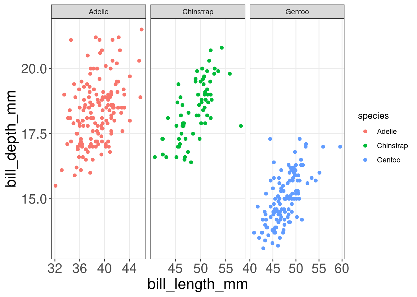

# do not do this if you are comparing facets via the y
# axis!

12.2 Facetting by two variables

ggplot(data = penguins) + geom_point(aes(x = bill_length_mm,
    y = bill_depth_mm, colour = species)) + facet_grid(year ~
    species, scales = "free")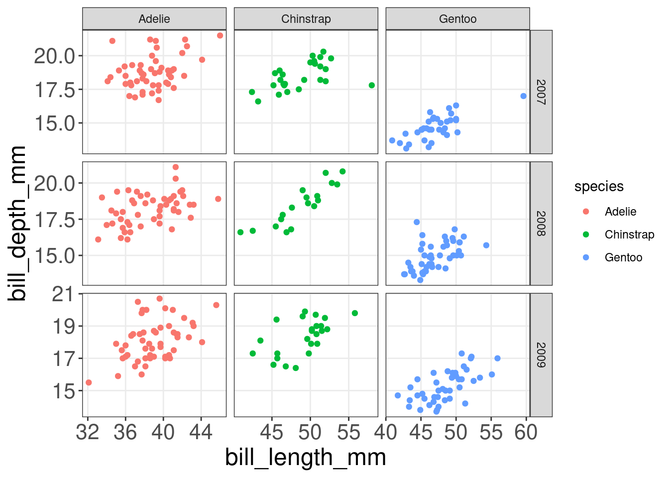

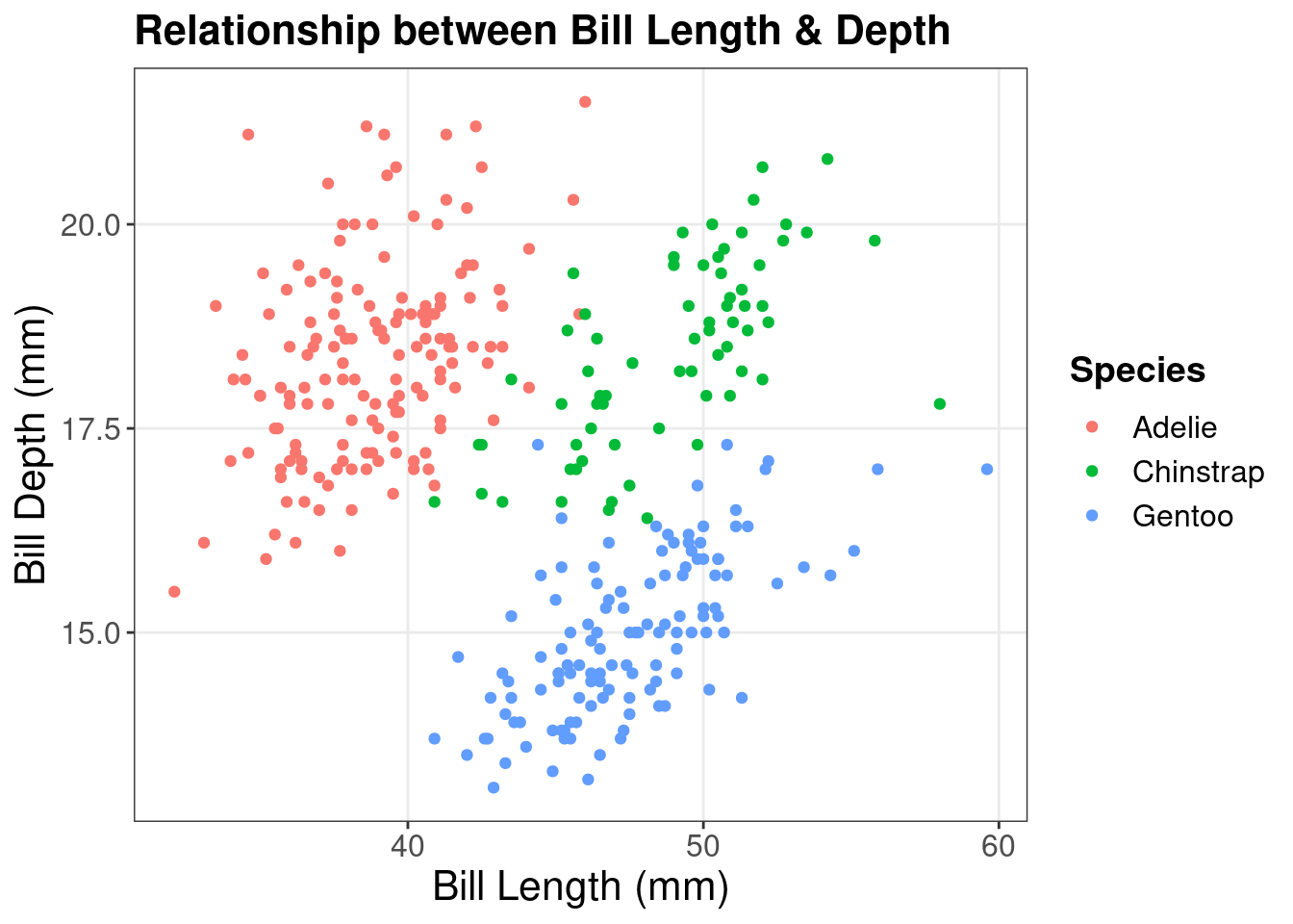
12.3 Title and axes components: size, colour and face

Let us come back to our default plot that we have been building on.

# Let's come back to our penguin plot from before
pp

We can tune the axes and titles to make the information clearer, so the plot can speak for itself.

12.4 Challenge 3

Use the tips dataset found in reshape2 📦 to reproduce the plot below.

# install and load the package
install.packages("reshape2")

## Installing package into '/home/runner/work/_temp/Library'
## (as 'lib' is unspecified)

library(reshape2)

Our tip: Go step by step! When fine-tuning your plot, start from theme_classic() and add theme() to make your additional changes.

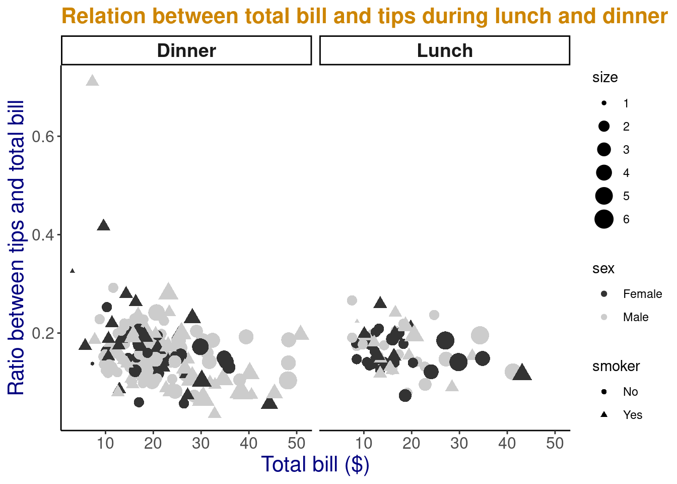
12.4.1 Challenge 3: Solution

# Build the plot
tips.gg <- ggplot(tips, 
                  # Step 1. Specify the aesthetic mapping from the axes and the legends
                  aes(x = total_bill,
                      y = tip/total_bill,
                      shape = smoker,
                      colour = sex,
                      size = size)) +
  # Step 2. Specify the geom used to represent the data
  geom_point() +
  # Step 3. Specify the variable used to make facets
  facet_grid( ~ time) +
  # Step 4. set the colour scale used to represent sex 
  scale_colour_grey() +
  # Step 5. Label the plot title and axes
  labs(title = "Relation between total bill and tips during lunch and dinner",
       x = "Total bill ($)", 
       y = "Ratio between tips and total bill") +
  # Step 6. Set the theme
  theme_classic() +
  # Step 7. Customise the theme to match the sizing and colour of the plot labels
  theme(axis.title = element_text(size = 16,
                                  colour = "navy"),
        axis.text = element_text(size = 12),
        plot.title = element_text(size = 16,
                                  colour = "orange3",
                                  face = "bold"),
        # this part adjusts the text in the facet labels (strips!)
        strip.text.x = element_text(size = 14, face="bold"))
# print our beautiful plot!
tips.gg