Chapter 5 Grammar of Graphics (GG) basics

5.1 What is the Grammar of Graphics?

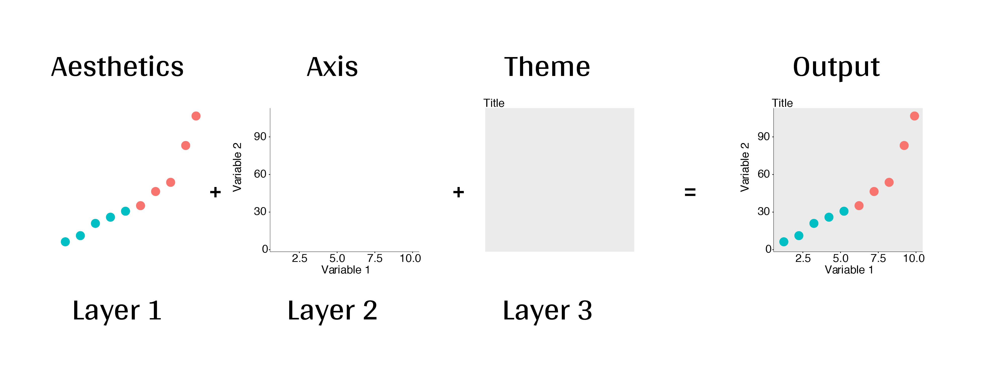
Let’s start with the basics! The package ggplot2 is based on the Grammar of Graphics (GG), which is a framework for data visualization that dissects each component of a graph into individual components, creating distinct layers. Using the GG system, we can build graphs step-by-step for flexible, customizable results.

GG layers have specific names that you will see throughout the workshop:

Figure 5.1: Image adapted from The Grammar of Graphics.

To make a ggplot, the data and mapping layers are basic requirements, while the other layers are for additional customization. The layers that are “not required” are still important to think about, but you will be able to generate a basic plot without them.

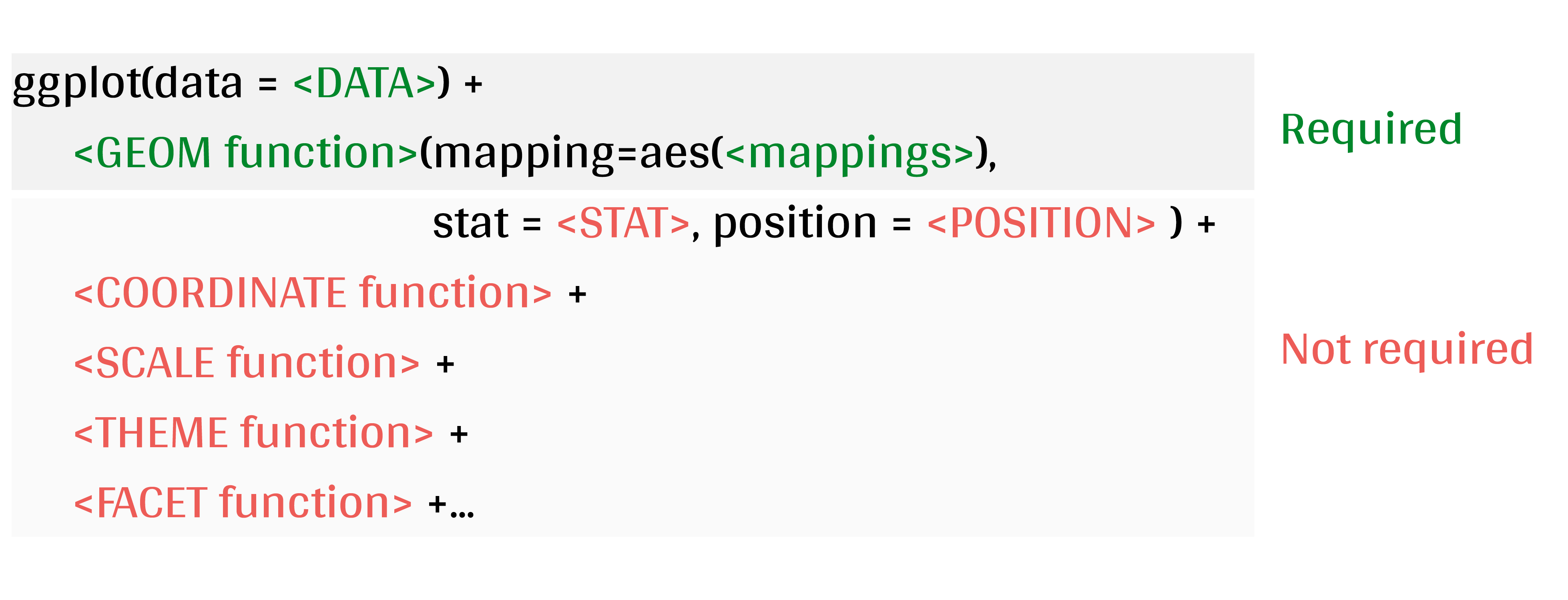
Figure 5.2: Basic requirements to generate a ggplot.

5.2 Grammar of Graphics layers

5.2.1 A breakdown of common layers

Here is a breakdown of each Grammar of Graphics layer and common arguments for each that can be used as a reference:

• Data:
  • your data, in tidy format, will provide ingredients for your plot
  • use dplyr techniques to prepare data for optimal plotting format
  • usually, this means you should have one row for every observation that you want to plot
• Aesthetics (aes), to make data visible
  • x, y: variable along the x and y axis
  • colour: color of geoms according to data
  • fill: the inside color of the geom
  • group: what group a geom belongs to
  • shape: the figure used to plot a point
  • linetype: the type of line used (solid, dashed, etc)
  • size: size scaling for an extra dimension
  • alpha: the transparency of the geom
• Geometric objects (geoms - determines the type of plot)
  • geom_point(): scatterplot
  • geom_line(): lines connecting points by increasing value of x
  • geom_path(): lines connecting points in sequence of appearance
  • geom_boxplot(): box and whiskers plot for categorical variables
  • geom_bar(): bar charts for categorical x axis
  • geom_histogram(): histogram for continuous x axis
  • geom_violin(): distribution kernel of data dispersion
  • geom_smooth(): function line based on data
• Facets
  • facet_wrap() or facet_grid() for small multiples
• Statistics
  • similar to geoms, but computed
  • show means, counts, and other statistical summaries of data
• Coordinates - fitting data onto a page
  • coord_cartesian to set limits
  • coord_polar for circular plots
  • coord_map for different map projections
• Themes
  • overall visual defaults
  • fonts, colors, shapes, outlines

5.2.2 Putting these layers together

Let’s try it out! Here are the basic steps to build a plot. You can refer back to these steps throughout the workshop if you need help!

1. Create a simple plot object:

• plot.object <- ggplot()

2. Add geometric layers:

• plot.object <- plot.object + geom_*()

3. Add appearance layers:

• plot.object <- plot.object + coord_*() + theme()

3. Repeat step 2-3 until satisfied, then print:

• plot.object or print(plot.object)

We will come back to this syntax in Chapter 6.4, where we work through the layers in greater depth!

---

All the content of the workshop series is under a Creative Commons Attribution-NonCommercial-ShareAlike 4.0 International License.