Chapter 11 Step 3. Model validation

Now that we have our model, we must verify that the model follows all the basic assumptions:

1. Check the homogeneity of the variance:
- Plot predicted values vs residual values
2. Check the independence of the model residuals:
- Plot residuals vs each covariate of the model
- Plot residuals vs each covariate not included in the model
3. Check the normality of the model residuals:
- Histogram of residuals

11.1 1. Check the homogeneity of the variance

In order to check the homgeneity of the variance, we can plot predicted values vs residual values.

Homogeneous dispersion of the residuals means that the assumption is respected.

Now let’s look at our data, is the dispersion homogenous?

# Plot predicted values vs residual values
par(mar = c(4, 4, 0.5, 0.5))
plot(resid(M8) ~ fitted(M8), xlab = "Predicted values", ylab = "Normalized residuals")
abline(h = 0, lty = 2)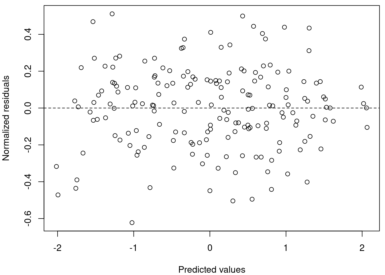

# Homogeneous dispersion of the residuals means that the
# assumption is respected.

Yes! Homogeneous dispersion of the residuals means that the assumption is respected.

11.2 2. Check the independence of the model residuals with each covariate

In order to check the independence of the model residuals with each covariate we will (1) plot residuals vs each covariate of the model and (2) plot residuals vs each covariate not included in the model.

Let’s start by (1) plotting the residuals vs each covariate of the model.

# In order to check the independence of the model residuals
# we need to plot residuals vs each covariate of the model
par(mfrow = c(1, 3), mar = c(4, 4, 0.5, 0.5))

plot(resid(M8) ~ fish.data$Z_Length, xlab = "Length", ylab = "Normalized residuals")
abline(h = 0, lty = 2)

boxplot(resid(M8) ~ Fish_Species, data = fish.data, xlab = "Species",
    ylab = "Normalized residuals")
abline(h = 0, lty = 2)

boxplot(resid(M8) ~ Lake, data = fish.data, xlab = "Lakes", ylab = "Normalized residuals")
abline(h = 0, lty = 2)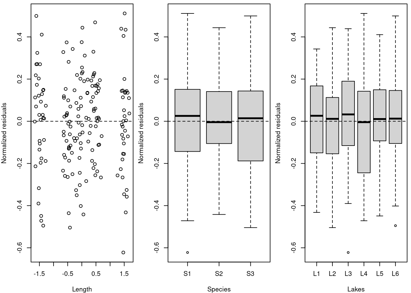

# Homogeneous dispersion of the residuals around 0 means no
# pattern of residuals depending on the variable, therefore
# the assumption is respected!  Note: The clusters are due
# to the data structure, where fish of only 5 size classes
# (large, small, and three groups in between) were
# captured.

Homogeneous dispersion of the residuals around 0 means no pattern of residuals depending on the variable, therefore the assumption is respected!

Note: The clusters are due to the data structure, where fish of only 5 size classes (large, small, and three groups in between) were captured.

Now, we should (2) plot residuals vs each covariate not included in the model.

If you observe patterns in these plots, you will know that there is variation in your dataset that could be explained by these covariates and you should consider including them in your model. However because we have included all the measured variables in our model, we can not do this step with our data.

11.3 3. Check the normality of the model residuals

Now we will check the normality of the model residuals as residuals following a normal distribution indicate that the model is not biased.

# Check the normality of the model residuals as residuals
# following a normal distribution indicate that the model
# is not biased.
hist(resid(M8))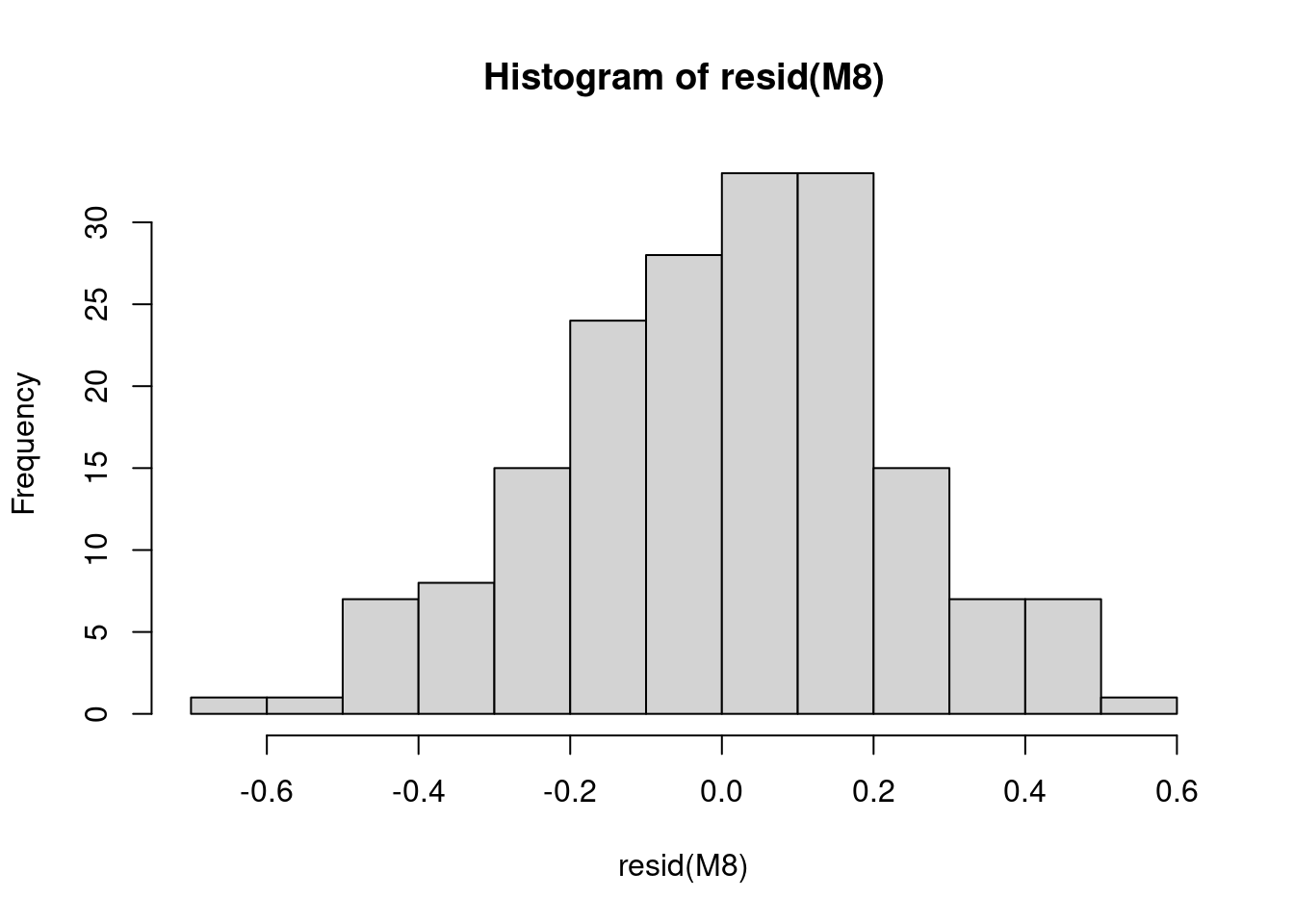

# The residuals are normal! This means our model is not
# biased.

The residuals are normal! This means our model is not biased.