Chapter 4 Starting with a question

Before we dive in, let’s start by considering an example dataset and proposing a research question.

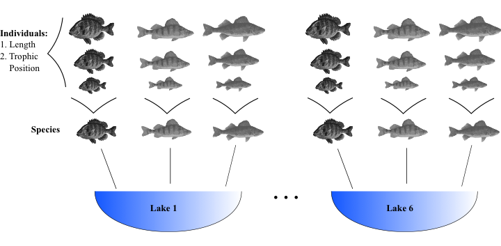
The dataset we will be using looks at fish trophic positions. In this dataset, data was collected for 3 different fish species (S1-3) with 10 individuals sampled per species across 6 different lakes (L1-6). Individuals from each species were measured and exhibit variation in their body length and trophic position.

Here is a visual representation to help wrap your head around all of this!

Note: Only three sizes of fish are shown within each species but in reality there are 10 individuals per species.

A simple question you could answer with this dataset is: does fish trophic position increase with fish size? This will be our motivating question for this workshop.

4.1 Challenge 1

For our first challenge, we are going to start looking deeper at our dataset. Reproduce plots 1-3 using the script below and the fish dataset. Observe each plot and try to get a sense of what is occurring. A few key questions to ask yourself are:

1. Do we expect an increase in trophic position with length in the exact same way for all species?
2. Do we expect an increase in trophic position with length in the exact same way for all lakes?

How might these relationships differ?

library(ggplot2)
# Load the dataset
fish.data <- read.csv("data/qcbs_w7_data.csv", stringsAsFactors = TRUE)
# This line will vary depending on where your data is
# saved.  Check your working directory with getwd() and
# change it, if needed, with setwd()

# Simple theme for all ggplot figures we produce after this
fig <- theme_bw() + theme(panel.grid.minor = element_blank(),
    panel.grid.major = element_blank(), panel.background = element_blank(),
    strip.background = element_blank(), strip.text.y = element_text(),
    legend.background = element_blank(), legend.key = element_blank(),
    panel.border = element_rect(colour = "black", fill = NA))


# Exploring the data graphically!

# Basic plot aesthetics for the relationship we care about
plot <- ggplot(aes(Fish_Length, Trophic_Pos), data = fish.data)

# Plot 1 - All data
plot + geom_point() + labs(x = "Length (mm)", y = "Trophic position",
    title = "All data") + fig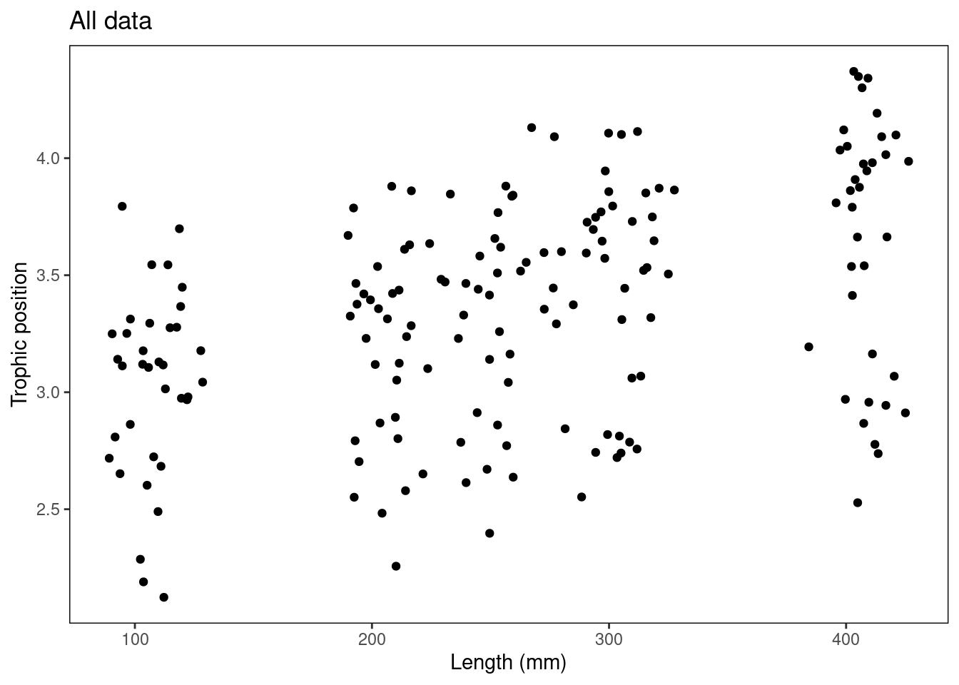

# Plot 2 - By species
plot + geom_point() + facet_wrap(~Fish_Species) + labs(x = "Length (mm)",
    y = "Trophic position", title = "By species") + fig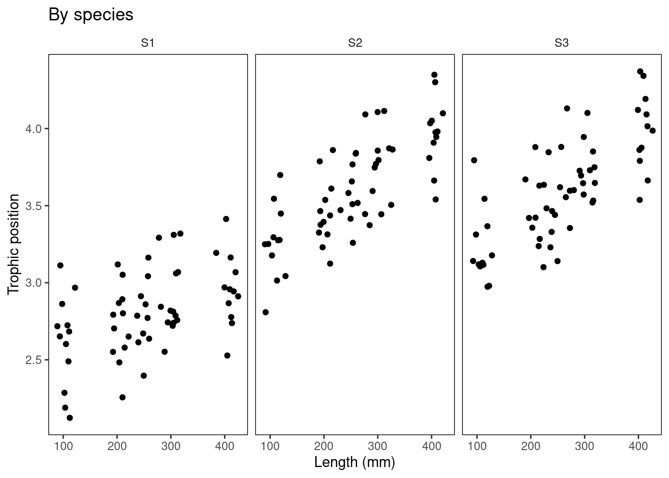

# Plot 3 – By lake
plot + geom_point() + facet_wrap(~Lake) + labs(x = "Length (mm)",
    y = "Trophic position", title = "By lake") + fig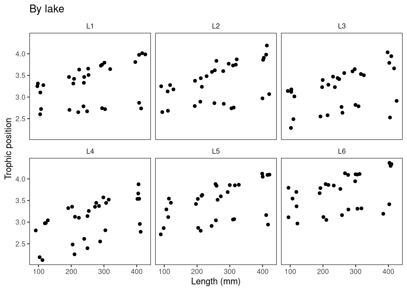

Challenge 1 Solution:

Based on these plots, we can draw two initial observations:

1. All species appear to increase in trophic position with length, but the slope might be different across species.

2. Some parameters specific to each particular lake (e.g. the system’s primary productivity) may change the observed relationship.