Chapter 11 Introduction to Generalized Additive Mixed Models (GAMMs)

When observations are not independent, GAMs can be used to either incorporate:

a correlation structure to model autocorrelated residuals, such as:
the autoregressive (AR) model
the moving average model (MA); or,
a combination of both models (ARMA).
random effects that model independence among observations from the same site using GAMMs.

That is, in addition to changing the basis as with the nottem example, we can also add complexity to the model by incorporating an autocorrelation structure or mixed effects using the gamm() function in the mgcv package. Although we will not be using it here, the gamm4 package can also be used to estimate GAMMs in R.

11.1 Residual autocorrelation

Autocorrelation of residuals refers to the degree of correlation between the residuals (the differences between the actual and predicted values) in a time series model.

In other words, if there is an autocorrelation of residuals in a time series model, it means that there is a pattern or relationship between the residuals at one point in time and the residuals at other points in time.

Autocorrelation of residuals is usually measured using the ACF (autocorrelation function) and pACF (partial autocorrelation function) graphs, which show the correlation between residuals at different lags.

11.1.0.1 The autocorrelation function

The autocorrelation function (ACF) of a stationary time series can be defined using the following equation:

\[ACF(k) = Corr(Y_t, Y_{t-k})\] where \(Y_t\) is the value of the time series at time \(t\), \(Y_{t-k}\) is the value of the time series at time \(t-k\), and \(Corr()\) is the correlation coefficient between two random variables.

In other words, the ACF(\(k\)) is the correlation between the values of the time series \(Y_t\) and \(Y_{t-k}\), where \(k\) is the lag between the two points in time. The ACF is a measure of the strength of the correlation between each value in the time series and its lagged values at different times.

11.1.0.2 The partial autocorrelation function

The partial autocorrelation function (pACF) of a stationary time series can be defined using the following recursive formula:

\[pACF(1) = Corr(Y_1, Y_2)\]

\[pACF(k) = [ Corr(Y_k, Y_{k+1} - \hat{\phi}{k,1}Y{k}) ] / [ Corr(Y_1, Y_2 - \hat{\phi}_{1,1}Y_1) ]\]

for \(k > 1\)

where \(Y_t\) is the value of the time series at time \(t\), \(\hat{\phi}{k,1}\), \(\hat{\phi}{1,1}\), \(...\) \(\hat{\phi}{k-1,k-1}\) are the coefficients of the autoregressive model of order \(k-1\) fitted to the time series, and \(Corr()\) is the coefficient of correlation between two random variables

In other words, the pACF(\(k\)) is the correlation between the values of the time series \(Y_k\) and \(Y_{k+j}\) after removing the influence of intermediate lags \(Y_{k+1}, Y_{k+2}, ..., Y_{k+j-1}\) using an autoregressive model of order \(k-1\). The pACF measures the correlation between \(Y_k\) and \(Y_{k+j}\) after removing the effect of any shorter intermediate lags.

If the ACF or pACF graphs show significant correlations at non-zero lags, there is evidence of autocorrelation in the residuals and the model may need to be modified or improved to better capture the underlying patterns in the data.

Let’s see how this works with our year_gam model!

To start, let’s have a look at a model with temporal autocorrelation in the residuals. We will revisit the Nottingham temperature model and test for correlated errors using the (partial) autocorrelation function.

par(mfrow = c(1, 2))
acf(resid(year_gam), lag.max = 36, main = "ACF")
pacf(resid(year_gam), lag.max = 36, main = "pACF")

The autocorrelation function (ACF; first panel above) evaluates the cross correlation of a time series with itself at different time lags (i.e. similarity between observations at increasingly large time lags).

In contrast, the partial autocorrelation function (PACF: second panel above) gives the partial correlation of a time series with its own lagged values, after controlling for the values of the time series at all shorter lags.

The ACF and pACF plots are thus used to identify the time steps are needed before observations are no longer autocorrelated.

11.2 Generalized additive mixed effect models (GAMMs) in a nutshell

Generalized additive mixed effect models (GAMMs) are a type of statistical model that combines the flexibility of generalized additive models (GAMs) with the ability to account for random effects in mixed-effect models.

Like GAMs, GAMMs allow for non-linear relationships between predictors and the response variable by fitting smooth functions to each predictor. However, GAMMs also allow for the inclusion of random effects, which capture the variability of observations within groups or clusters.

A generalized additive mixed effects model (GAMM) can be written as:

\[Y_i = f_1(X_{1,i}) + f_2(X_{2,i}) + \ldots + f_p(X_{p,i}) + Z_i b + \epsilon_i\]

In this formula, \(Y_i\) represents the response variable for the \(i\)th observation, and \(X_{1,i}\) to \(X_{p,i}\) represent the values of the \(p\) predictor variables for that observation. The functions \(f_1\) to \(f_p\) represent the relationships between each predictor variable and the response variable.

The term \(Z_i b\) represents the random effects in the model. \(Z_i\) is a matrix that specifies the random effects design for the \(i\)th observation, and \(b\) is a vector of random effects coefficients.

Finally, \(\epsilon_i\) represents the error term for the \(i\)th observation.

11.2.1 Application

The ACF plot of our model residuals suggests a significant lag of 1, and perhaps a lag of 2. Therefore, a low-order AR model is likely needed.

We can test this by adding AR structures to the Nottingham temperature model. Let’s make one with an AR(1) (correlation at 1 time step) and one with an AR(2) (correlation at two times steps), and compare models using AIC to find a the best-fit model.

df <- data.frame(nottem, nottem_year, nottem_month)

year_gam <- gamm(nottem ~ s(nottem_year) + s(nottem_month, bs = "cc"),
    data = df)

year_gam_AR1 <- gamm(nottem ~ s(nottem_year) + s(nottem_month,
    bs = "cc"), correlation = corARMA(form = ~1 | nottem_year,
    p = 1), data = df)

year_gam_AR2 <- gamm(nottem ~ s(nottem_year) + s(nottem_month,
    bs = "cc"), correlation = corARMA(form = ~1 | nottem_year,
    p = 2), data = df)

Which of these models performs the best?

AIC(year_gam$lme, year_gam_AR1$lme, year_gam_AR2$lme)

##                  df      AIC
## year_gam$lme      5 1109.908
## year_gam_AR1$lme  6 1101.218
## year_gam_AR2$lme  7 1101.598

The AR(1) provides a significant increase in fit over the naive model (year_gam), but there is very little improvement in moving to the AR(2). So, it is best to include only the AR(1) structure in our model.

11.3 Random effects

As we saw in the section about changing the basis, bs specifies the type of underlying base function. For random intercepts and linear random slopes we use bs = "re", but for random smooths we use bs = "fs".

There are three different types of random effects in GAMMs. Below, we use fac to indicate factor coding for the random effect, and x0 for a continuous fixed effect:

Random intercepts adjust the height of other model terms with a constant value: s(fac, bs = "re")
Random slopes adjust the slope of the trend of a numeric predictor: s(fac, x0, bs = "re")
Random smooths adjust the trend of a numeric predictor in a nonlinear way: s(x0, fac, bs = "fs", m = 1), where the argument m = 1 sets a heavier penalty for the smooth moving away from 0, causing shrinkage to the mean.

For more detailed explanations about random effects, see Workshop 7.

This is a (very!) brief overview of how you can use random effects in GAMMs. For further details, we really recommend Pedersen et al. (2019), which is a very accessible article outlining various ways to build GAMMs to answer ecological questions.

11.3.1 GAMM with a random intercept

We will use the gamSim() function to generate a dataset with a random effect, then run a model with a random intercept using fac as the random factor.

# generate and view data
gam_data2 <- gamSim(eg = 6)

## 4 term additive + random effectGu & Wahba 4 term additive model

head(gam_data2)

##           y        x0         x1        x2        x3         f        f0
## 1  8.411980 0.7369989 0.30941786 0.5079422 0.5440523  9.066472 1.4707805
## 2  9.208443 0.1083441 0.34284917 0.6295774 0.3747799 11.956612 0.6676773
## 3 18.986368 0.9648756 0.24928256 0.4615991 0.3388980 13.867240 0.2202455
## 4 15.279170 0.8198440 0.03304455 0.5583043 0.6934456 17.072441 1.0724811
## 5 16.254626 0.3668214 0.48894089 0.2308583 0.1565436 16.404978 1.8274861
## 6 16.580965 0.8007808 0.67568426 0.6680502 0.5543013 14.247673 1.1715978
##         f1       f2 f3 fac
## 1 1.856765 2.738927  0   1
## 2 1.985158 3.303777  0   2
## 3 1.646357 3.000637  0   3
## 4 1.068322 2.931638  0   4
## 5 2.658818 8.918673  0   1
## 6 3.862708 3.213367  0   2

# run random intercept model
gamm_intercept <- gam(y ~ s(x0) + s(fac, bs = "re"), data = gam_data2,
    method = "REML")

# examine model output
summary(gamm_intercept)$s.table

##             edf   Ref.df         F     p-value
## s(x0)  3.245961 4.039044  4.565478 0.001298306
## s(fac) 2.966403 3.000000 88.124739 0.000000000

Note that there is now a smoother term for the random intercept in the summary table. You can plot and view the random intercepts for each level of fac as follows:

plot(gamm_intercept, select = 2)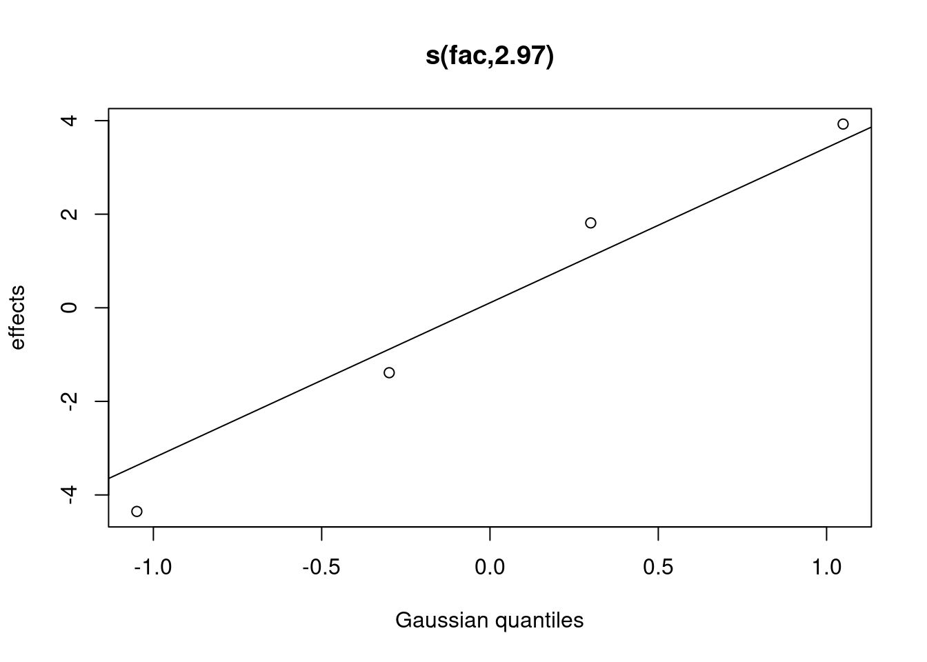

# select = 2 because the random effect appears as the
# second entry in the summary table.

We can also use the plot_smooth function to visualize the model, which allows us to plot a smooth of the summed effects of a GAM (based on predictions). This function also optionally removes the random effects by setting rm.ranef = TRUE.

Here, we will plot the summed effects for the x0 without random effects, and then plot the predictions of all four levels of the random fac effect:

par(mfrow = c(1, 2), cex = 1.1)

# Plot the summed effect of x0 (without random effects)
plot_smooth(gamm_intercept, view = "x0", rm.ranef = TRUE, main = "intercept + s(x1)")

# Plot each level of the random effect
plot_smooth(gamm_intercept, view = "x0", rm.ranef = FALSE, cond = list(fac = "1"),
    main = "... + s(fac)", col = "orange", ylim = c(0, 25))
plot_smooth(gamm_intercept, view = "x0", rm.ranef = FALSE, cond = list(fac = "2"),
    add = TRUE, col = "red")
plot_smooth(gamm_intercept, view = "x0", rm.ranef = FALSE, cond = list(fac = "3"),
    add = TRUE, col = "purple")
plot_smooth(gamm_intercept, view = "x0", rm.ranef = FALSE, cond = list(fac = "4"),
    add = TRUE, col = "turquoise")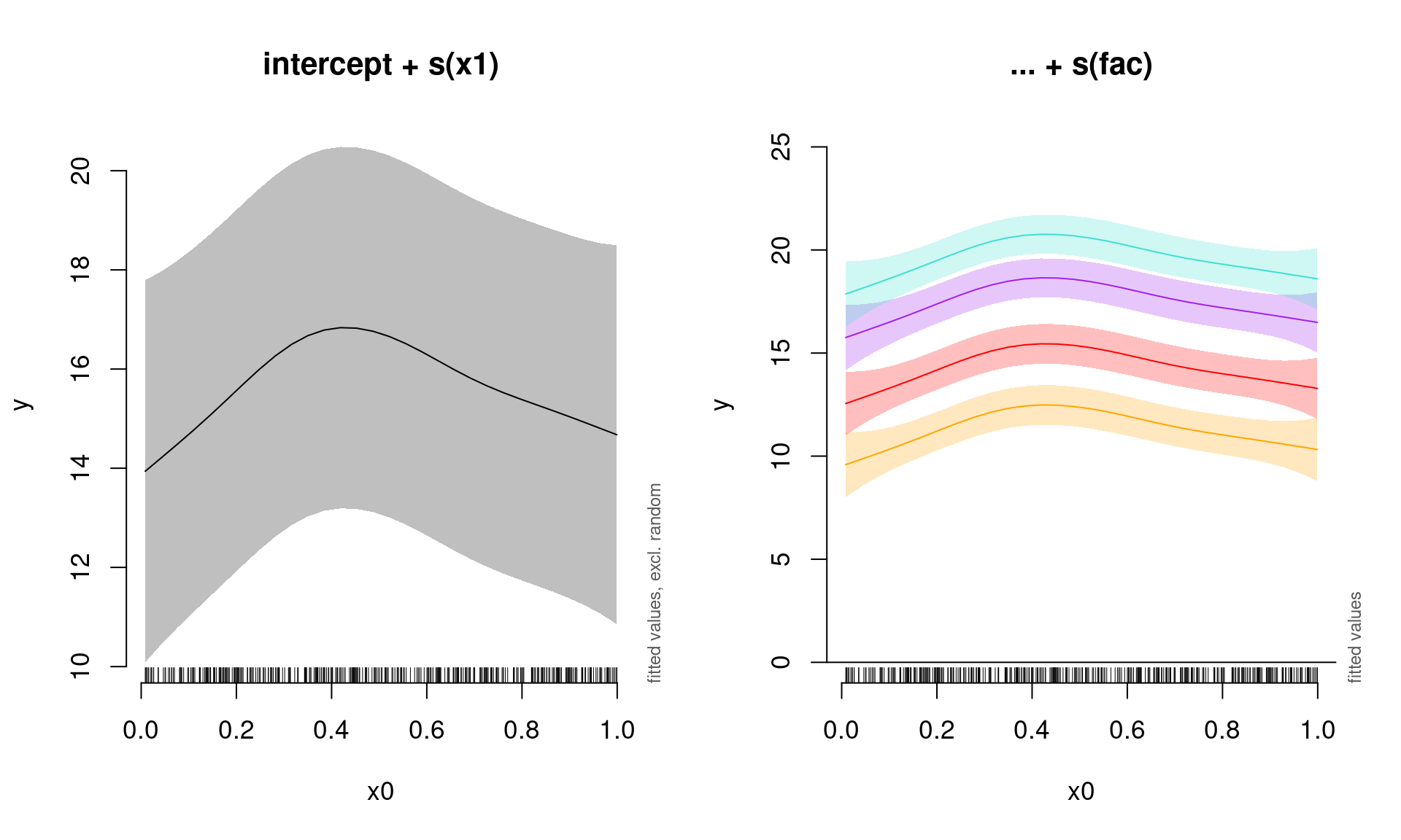

11.3.2 GAMM with a random slope

Next, we will run and plot a model with a random slope:

gamm_slope <- gam(y ~ s(x0) + s(x0, fac, bs = "re"), data = gam_data2,
    method = "REML")

summary(gamm_slope)$s.table

##                edf   Ref.df         F      p-value
## s(x0)     3.291985 4.095352  5.142403 0.0004551535
## s(x0,fac) 2.949291 3.000000 56.637107 0.0000000000

We can once again plot the summed effects for the x0 without random effects, and then plot the predictions of all four levels of the random fac effect:

par(mfrow = c(1, 2), cex = 1.1)

# Plot the summed effect of x0 (without random effects)
plot_smooth(gamm_slope, view = "x0", rm.ranef = TRUE, main = "intercept + s(x1)")

# Plot each level of the random effect
plot_smooth(gamm_slope, view = "x0", rm.ranef = FALSE, cond = list(fac = "1"),
    main = "... + s(fac, x0)", col = "orange", ylim = c(0, 25))
plot_smooth(gamm_slope, view = "x0", rm.ranef = FALSE, cond = list(fac = "2"),
    add = TRUE, col = "red")
plot_smooth(gamm_slope, view = "x0", rm.ranef = FALSE, cond = list(fac = "3"),
    add = TRUE, col = "purple")
plot_smooth(gamm_slope, view = "x0", rm.ranef = FALSE, cond = list(fac = "4"),
    add = TRUE, col = "turquoise")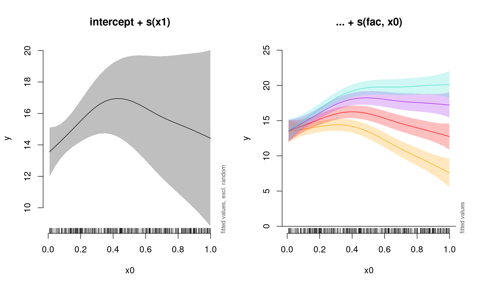

11.3.3 GAMM with a random intercept and slope

We will now include both a random intercept and a random slope term.

gamm_int_slope <- gam(y ~ s(x0) + s(fac, bs = "re") + s(fac,
    x0, bs = "re"), data = gam_data2, method = "REML")

summary(gamm_int_slope)$s.table

##                    edf   Ref.df            F     p-value
## s(x0)     3.2459692005 4.039052 4.565467e+00 0.001298329
## s(fac)    2.9663722096 3.000000 8.817810e+01 0.000000000
## s(fac,x0) 0.0006401119 3.000000 1.061841e-04 0.695560853

We can once again plot the summed effects for the x0 without random effects, and then plot the predictions of all four levels of the random fac effect:

par(mfrow = c(1, 2), cex = 1.1)

# Plot the summed effect of x0 (without random effects)
plot_smooth(gamm_int_slope, view = "x0", rm.ranef = TRUE, main = "intercept + s(x1)")

# Plot each level of the random effect
plot_smooth(gamm_int_slope, view = "x0", rm.ranef = FALSE, cond = list(fac = "1"),
    main = "... + s(fac) + s(fac, x0)", col = "orange", ylim = c(0,
        25))
plot_smooth(gamm_int_slope, view = "x0", rm.ranef = FALSE, cond = list(fac = "2"),
    add = TRUE, col = "red")
plot_smooth(gamm_int_slope, view = "x0", rm.ranef = FALSE, cond = list(fac = "3"),
    add = TRUE, col = "purple")
plot_smooth(gamm_int_slope, view = "x0", rm.ranef = FALSE, cond = list(fac = "4"),
    add = TRUE, col = "turquoise")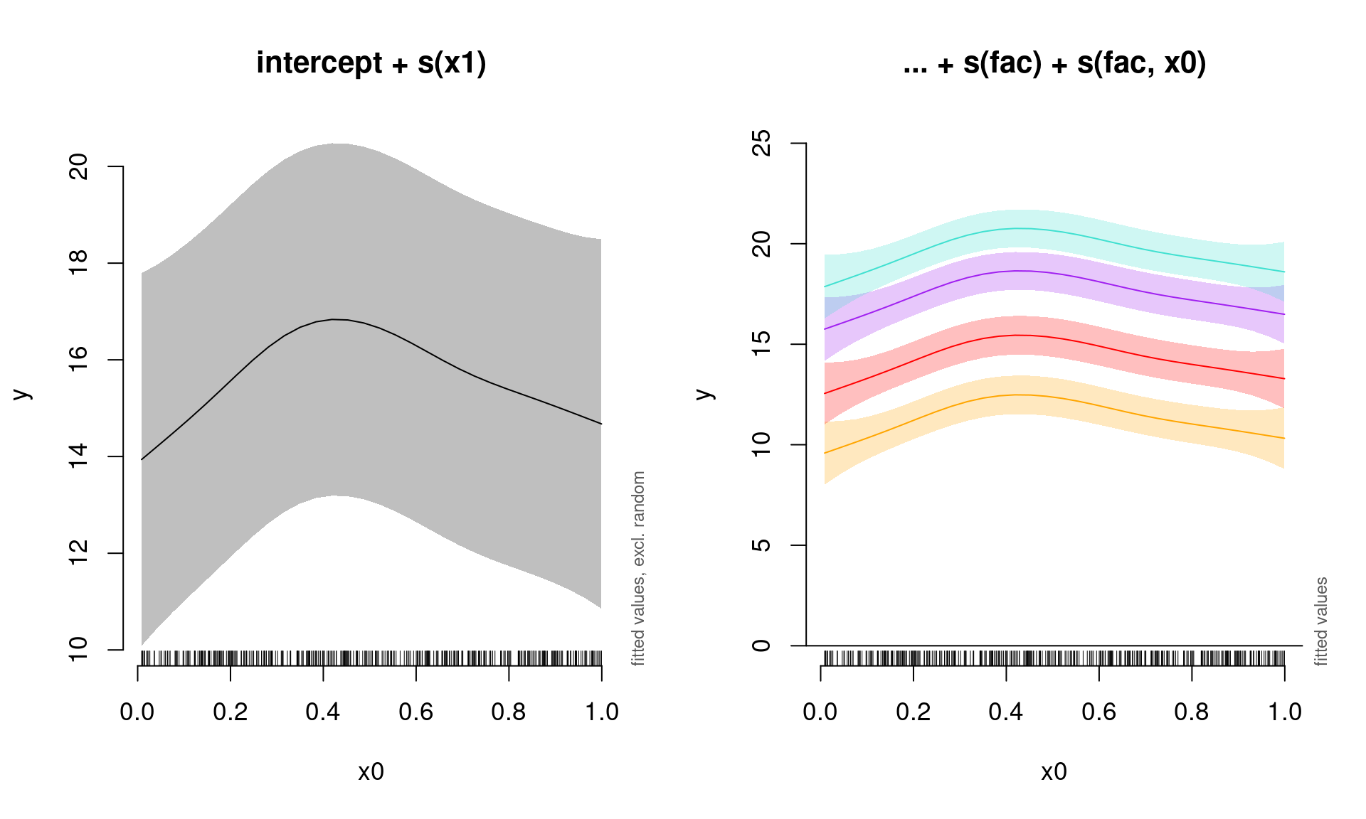

Note that the random slope is static in this case:

plot(gamm_int_slope, select = 3)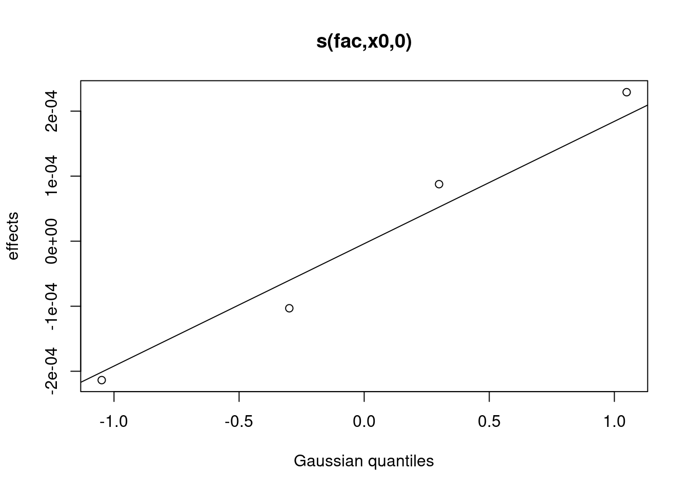

# select = 3 because the random slope appears as the third
# entry in your summary table.

11.3.4 GAMM with a random smooth

Lastly, we will examine a model with a random smooth.

gamm_smooth <- gam(y ~ s(x0) + s(x0, fac, bs = "fs", m = 1),
    data = gam_data2, method = "REML")

## Warning in gam.side(sm, X, tol = .Machine$double.eps^0.5): model has repeated
## 1-d smooths of same variable.

summary(gamm_smooth)$s.table

##                edf    Ref.df        F     p-value
## s(x0)     3.245946  4.039007 4.565087 0.001299197
## s(x0,fac) 2.968037 35.000000 7.553585 0.000000000

Here, if the random slope varied along x0, we would see different curves for each level:

plot(gamm_smooth, select = 1)
# select = 1 because the smooth slope appears as the first
# entry in your summary table.

We can once again plot the summed effects for the x0 without random effects, and then plot the predictions of all four levels of the random fac effect:

par(mfrow = c(1, 2), cex = 1.1)

# Plot the summed effect of x0 (without random effects)
plot_smooth(gamm_smooth, view = "x0", rm.ranef = TRUE, main = "intercept + s(x1)")

# Plot each level of the random effect
plot_smooth(gamm_smooth, view = "x0", rm.ranef = FALSE, cond = list(fac = "1"),
    main = "... + s(fac) + s(fac, x0)", col = "orange", ylim = c(0,
        25))
plot_smooth(gamm_smooth, view = "x0", rm.ranef = FALSE, cond = list(fac = "2"),
    add = TRUE, col = "red")
plot_smooth(gamm_smooth, view = "x0", rm.ranef = FALSE, cond = list(fac = "3"),
    add = TRUE, col = "purple")
plot_smooth(gamm_smooth, view = "x0", rm.ranef = FALSE, cond = list(fac = "4"),
    add = TRUE, col = "turquoise")

11.3.5 GAMM model comparison

All of the mixed models from this section can be compared using AIC() to determine the best fit model

AIC(gamm_intercept, gamm_slope, gamm_int_slope, gamm_smooth)

##                      df      AIC
## gamm_intercept 8.804002 2229.206
## gamm_slope     8.786560 2290.520
## gamm_int_slope 8.806546 2229.210
## gamm_smooth    8.810264 2229.216

The best model among those we have built here would be a GAMM with a random effect on the intercept.

References

Pedersen, Eric J, David L Miller, Gavin L Simpson, and Noam Ross. 2019. “Hierarchical Generalized Additive Models in Ecology: An Introduction with Mgcv.” PeerJ 7: e6876. https://doi.org/https://doi.org/10.7717/peerj.6876.