Chapter 9 Other distributions

We need a probability distribution that allows the variance to increase with the mean.

One family of distributions that has this property and that works well in a GAM is the Tweedie family. A common link function for Tweedie distributions is the \(log\).

As in a GLM, we can use the family = argument in gam() to fit models with other distributions (including distributions such as binomial, poisson, gamma etc.).

To get an overview of families available in mgcv:

`?`(family.mgcv)

9.1 Challenge 3

Fit a new model smooth_interact_tw with the same formula as the smooth_interact model, but with a distribution from the Tweedie family (instead of the Normal distribution) and log link function. You can do so by using family = tw(link = "log") inside gam().
Check the choice of k and the residual plots for the new model.
Compare smooth_interact_tw with smooth_interact. Which one would you choose?

As a reminder, here is our smooth_interact model:

# Hint!  Because the Normal distribution is the default
# setting, we have not specified the distribution in this
# workshop yet.

# Here is how we would write the model to specify the
# Normal distribution:

smooth_interact <- gam(Sources ~ Season + s(SampleDepth, RelativeDepth,
    k = 60), family = gaussian(link = "identity"), data = isit,
    method = "REML")

9.1.1 Challenge 3: Solution

1. First, let us fit a new model with the Tweedie distribution and a log link function.

smooth_interact_tw <- gam(Sources ~ Season + s(SampleDepth, RelativeDepth,
    k = 60), family = tw(link = "log"), data = isit, method = "REML")
summary(smooth_interact_tw)$p.table

##              Estimate Std. Error  t value      Pr(>|t|)
## (Intercept) 1.3126641 0.03400390 38.60333 8.446478e-180
## Season2     0.5350529 0.04837342 11.06089  1.961733e-26

summary(smooth_interact_tw)$s.table

##                                   edf   Ref.df        F p-value
## s(SampleDepth,RelativeDepth) 43.23949 51.57139 116.9236       0

2. Check the choice of k and the residual plots for the new model.

Next, we should check the basis dimension:

k.check(smooth_interact_tw)

##                              k'      edf  k-index p-value
## s(SampleDepth,RelativeDepth) 59 43.23949 1.015062  0.8125

We should also verify the residual plots, to verify whether the Tweedie distribution is appropriate:

par(mfrow = c(2, 2))
gam.check(smooth_interact_tw)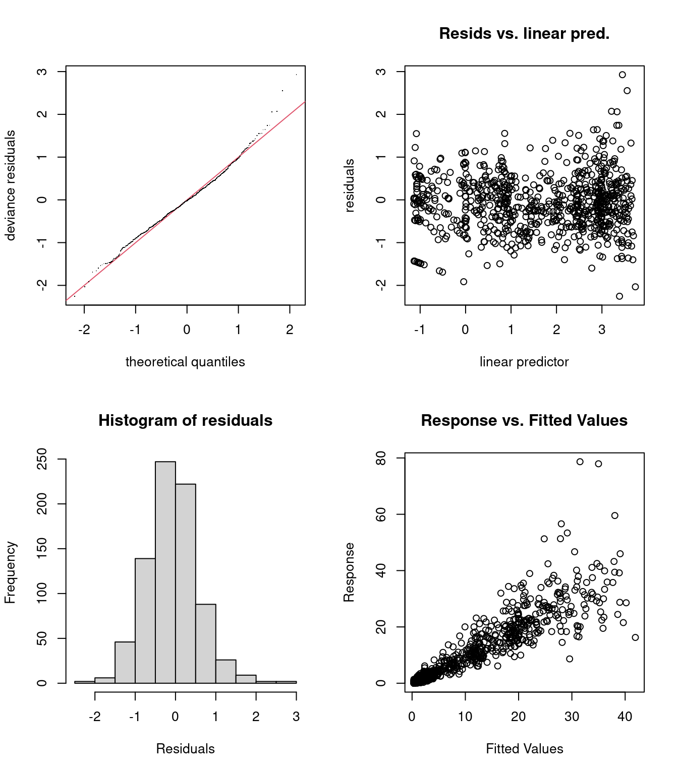

## 
## Method: REML   Optimizer: outer newton
## full convergence after 3 iterations.
## Gradient range [-0.0007646676,0.0001600484]
## (score 1791.138 & scale 0.4355231).
## Hessian positive definite, eigenvalue range [12.02444,492.4714].
## Model rank =  61 / 61 
## 
## Basis dimension (k) checking results. Low p-value (k-index<1) may
## indicate that k is too low, especially if edf is close to k'.
## 
##                                k'  edf k-index p-value
## s(SampleDepth,RelativeDepth) 59.0 43.2    1.02    0.88

The residual plots do look much better, but it is clear that something is missing from the model. This could be a spatial affect (longtitude and latitude), or a random effect (e.g. based on Station).

3. Compare smooth_interact_tw with smooth_interact. Which one would you choose?

AIC(smooth_interact, smooth_interact_tw)

##                          df      AIC
## smooth_interact    49.47221 4900.567
## smooth_interact_tw 47.86913 3498.490

AIC allows us to compare models that are based on different distributions!

The AIC score for smooth_interact_tw is much smaller than the AIC score for the smooth_interact. Using a Tweedie instead of a Normal distribution greatly improves our model!