Chapter 5 Loading, exploring and saving data
5.0.1 Working directory
R needs to know the directory where your data and files are stored in
order to load them. You can see which directory you are currently
working in by using the getwd() command.
getwd() # This commands shows the directory you are currently working inWhen you load a script, R automatically sets the working directory to the folder containing the script.
To change working directories using the setwd() function, specify the
working directory’s path using a “/” to separate folders, subfolders
and file names. You can also click Session > Set working directory >
Choose directory…
5.0.2 Display the content of the working directory
The command dir() displays the content of the working directory.
dir() # This command shows the content of the directory you are currently working inYou can check:
- Whether or not the file you plan to open is present in the current directory
- The correct spelling of the file name (e.g. ‘myfile.csv’ instead of ‘MyFile.csv’)
5.0.3 Importing data
Use the read.csv() command to import data in R.
CO2 <- read.csv("co2_good.csv") # Creates an object called CO2 by loading data from a file called 'co2_good.csv'This command specifies that you will be creating an R object named “CO2” by reading a csv file called “co2_good.csv”. This file must be located in your current working directory.
Recall that the question mark can be used to find out what arguments the function requires.
`?`(read.csv  # Use the question mark to pull up the help page for a command
)
In the help file you will note that adding the argument header=TRUE tells R that the first line of the spreadsheet contains column names and not data.
CO2 <- read.csv("co2_good.csv", header = TRUE)NOTE: If your operating system or CSV editor is in French, you may need
to use read.csv2() instead of read.csv()

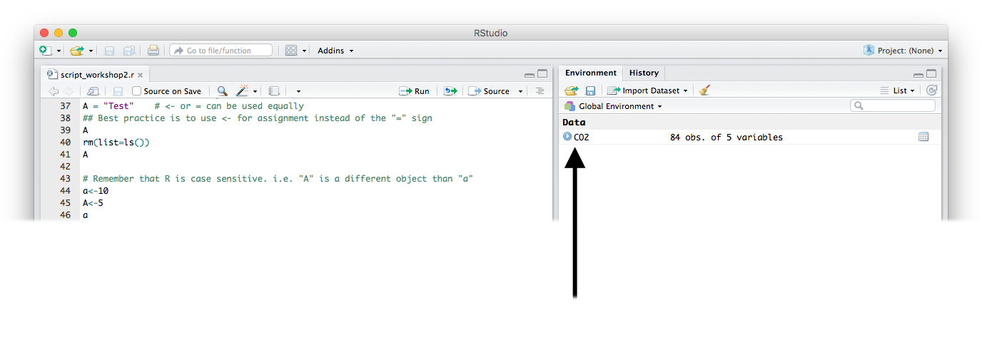
Notice that RStudio now provides information on the CO2 data in your workspace. The workspace refers to all the objects that you create during an R session.
5.0.4 Looking at data
The CO2 dataset consists of repeated measurements of CO2 uptake from six plants from Quebec and six plants from Mississippi at several levels of ambient CO2 concentration. Half of the plants of each type were chilled overnight before the experiment began.
There are some common commands that are useful to look at imported data:
| CO2 | Look at the whole data frame |
| head(CO2) | Look at the first few rows |
| tail(CO2) | Look at the last few rows |
| names(CO2) | Names of the columns in the data frame |
| attributes(CO2) | Attributes of the data frame |
| dim(CO2) | Dimensions of the data frame |
| ncol(CO2) | Number of columns |
| nrow(CO2) | Number of rows |
| summary(CO2) | Summary statistics |
| str(CO2) | Structure of the data frame |
The str() command is very useful to check the data type/mode for each
column (i.e. to check that all factors are factors, and numeric data is
stored as an integer or numeric. There are many common problems:
- Factors loaded as text (character) and vice versa
- Factors including too many levels because of a typo
- Numeric or integer data being loaded as a character due to a typo (including space or using a comma instead of a “.” for a decimal)
Exercise
Try to reload the data using:
CO2 <- read.csv("co2_good.csv", header = FALSE)Check the str() of CO2. What is wrong here? Reload the data with
header=TRUE before continuing.
5.0.5 Reminder from workshop 1: Accessing data
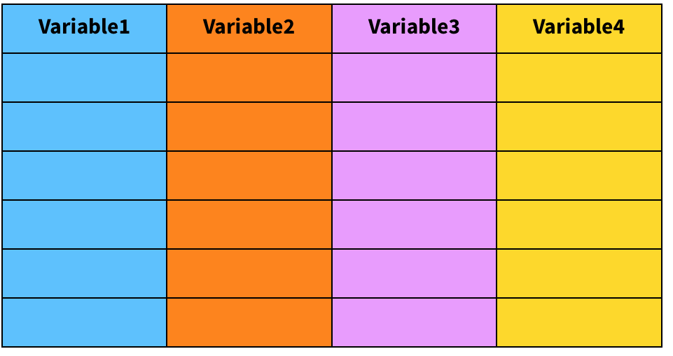
Data within a data frame can be extracted by several means. Let’s consider a data frame called mydata. Use square brackets to extract the content of a cell.

mydata[2, 3] # extracts the content of row 2 / column 3If column number is omitted, the whole row is extracted.
mydata[1, ] # extracts the content of the first rowThe squared brackets can also be used recursively
mydata[, 1][2] # this extracts the second content of the first columnIf row number is omitted, the whole column is extracted. Similarly, the
$ sign followed by the corresponding header can be used.
mydata$Variable1 # extracts a specific column by its name ('Variable1')5.0.6 Renaming variables
Variable names (i.e. column names) can be changed within R.
# First let's make a copy of the dataset to play with!
CO2copy <- CO2
# names() gives you the names of the variables present in
# the data frame
names(CO2copy)

# Changing from English to French names (make sure you have
# the same levels!)
names(CO2copy) <- c("Plante", "Categorie", "Traitement", "conc",
    "absortion")
5.0.7 Creating new variables
New variables can be easily created and populated. For example,
variables and strings can be concatenated together using the function
paste().
# Let's create an unique id for our samples using the
# function paste() see ?paste and ?paste0 Don't forget to
# use '' for strings
CO2copy$uniqueID <- paste0(CO2copy$Plante, "_", CO2copy$Categorie,
    "_", CO2copy$Traitement)

# Observe the results
head(CO2copy$uniqueID)
Creating new variables works for numbers and mathematical operations as well!
# Let's standardize our variable 'absortion' to relative
# values
CO2copy$absortionRel = CO2copy$absortion/max(CO2copy$absortion)  # Changing to relative values

# Observe the results
head(CO2copy$absortionRel)
5.0.8 Subsetting data
There are many ways to subset a data frame.
# Let's keep working with our CO2copy data frame

## Subsetting by variable name
CO2copy[, c("Plante", "absortionRel")]  # Selects only 'Plante' and 'absortionRel' columns. (Don't forget the ','!)

## Subsetting by row
CO2copy[1:50, ]  # Subset data frame from rows from 1 to 50

### Subsetting by matching with a factor level
CO2copy[CO2copy$Traitement == "nonchilled", ]  # Select observations matching only the nonchilled Traitement.

### Subsetting according to a numeric condition
CO2copy[CO2copy$absortion >= 20, ]  # Select observations with absortion higher or equal to 20

### Conditions can be complimentary -The & (and) argument-
CO2copy[CO2copy$Traitement == "nonchilled" & CO2copy$absortion >=
    20, ]

# We are done playing with the dataset copy. Let's erase
# it.
rm(CO2copy)
Go here to check all the logical operators you can use to subset a data frame in R
5.0.9 Data exploration
A good way to start your data exploration is to look at some basic
statistics of your dataset using the summary() function.
summary(CO2) # Get summary statistics of your datasetYou can also use some other functions to calculate basic statistics
about specific parts of your data frame, using mean(), sd(),
hist(), and print().
# Calculate mean and standard deviation of the
# concentration, and assign them to new variables
meanConc <- mean(CO2$conc)
sdConc <- sd(CO2$conc)

# print() prints any given value to the R console
print(paste("the mean of concentration is:", meanConc))
print(paste("the standard deviation of concentration is:", sdConc))

# Let's plot a histogram to explore the distribution of
# 'uptake'
hist(CO2$uptake)

# Increasing the number of bins to observe better the
# pattern
hist(CO2$uptake, breaks = 40)
The function apply() can be used to apply a function to multiple
columns of your data simultaneously. Use the ?apply command to get
more information about apply().
`?`(apply)To use apply, you have to specify three arguments. The first argument is the data you would like to apply the function to; the second argument is whether you would like to calculate based on rows (1) or columns (2) of your dataset; the third argument is the function you would like to apply. For example:
apply(CO2[, 4:5], MARGIN = 2, FUN = mean) # Calculate mean of the two columns in the data frame that contain continuous data5.0.10 Save your workspace
By saving your workspace, you can save the script and the objects
currently loaded into R. If you save your workspace, you can reload all
of the objects even after you use the rm(list=ls()) command to delete
everything in the workspace.
Use save.image() to save the workplace:
save.image(file = "co2_project_Data.RData")  # Save workspace

rm(list = ls())  # Clears R workspace

load("co2_project_Data.RData")  #Reload everything that was in your workspace

head(CO2)  # Looking good! :)