Chapter 15 Principal Coordinates Analysis

PCA as well as CA impose the distance preserved among objects: the Euclidean distance (and several others with pre-transformations) for PCA and the Chi2 distance for CA. If one wishes to ordinate objects on the basis of another distance measure, more appropriate to the problem at hand, then PCoA is the method of choice. In PCA we rotated and plotted our data so that as much variation was explained by a first Principal Component and we can see how much “species”, either actual species or environmental variables, contribute to each component by looking at the scores (also called “loadings”). Another type of unconstrained ordination is called Principal Coordinate Analysis (PCoA). In PCoA, points are added to plane space one at a time using Euclidean distance (or whatever distance (dissimilarity) metric you choose). Basically, one point is added, then a second so that it’s distance is correct from the first point and then the third point and so on adding as many axes (dimensions) as necessary along the way. Choosing between PCA and PCoA can be tricky, but generally PCA is used to summarize multivariate data into as few dimensions as possible, whereas PCoA can be used to visualize distances between points. PCoA can be particularly suited for datasets that have more columns than rows. For example, if hundreds of species have been observed over a set of quadrats, then a approach based on a PCoA using Bray-Curtis similarity (see below) may be best suited.

Run a PCoA on the Hellinger transformed species abundances (back to DoubsSpe):

# Using cmdscale() ?cmdscale cmdscale(dist(spe.hel),
# k=(nrow(spe)-1), eig=TRUE)

# Using pcoa()
`?`(pcoa)
spe.h.pcoa <- pcoa(dist(spe.hel))

# Extract the results spe.h.pcoa

# Construct the biplot
biplot.pcoa(spe.h.pcoa, spe.hel, dir.axis2 = -1)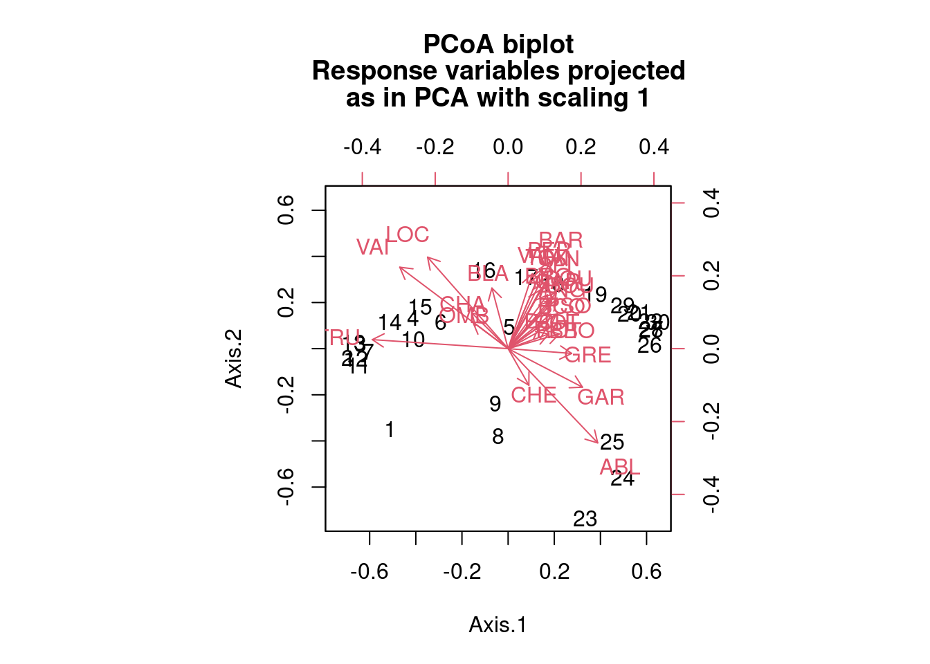

The output looks like this (and here here is a video that might help with the explanation of eigenvalues in terms of ordination).

You can also run a PCoA using a different distance measure (e.g. Bray-Curtis). Here is a PCoA run on a Bray-Curtis dissimilarity matrix:

spe.bray.pcoa <- pcoa(spe.db)  #where spe.db is the species dissimilarity matrix using Bray-Curtis. 
# spe.bray.pcoa

biplot.pcoa(spe.bray.pcoa, spe.hel, dir.axis2 = -1)

# Note that the distance measure chosen strongly influences
# the results.

Challenge 5 Run a PCoA on the Hellinger-transformed mite species abundance data. What are the significant axes? Which groups of sites can you identify? Which species are related to each group of sites? How do the PCoA results compare with the PCA results?

Challenge 5 - Solution Your code likely looks something like this:

mite.spe.h.pcoa <- pcoa(dist(mite.spe.hel))
# mite.spe.h.pcoa

biplot.pcoa(mite.spe.h.pcoa, mite.spe.hel, dir.axis2 = -1)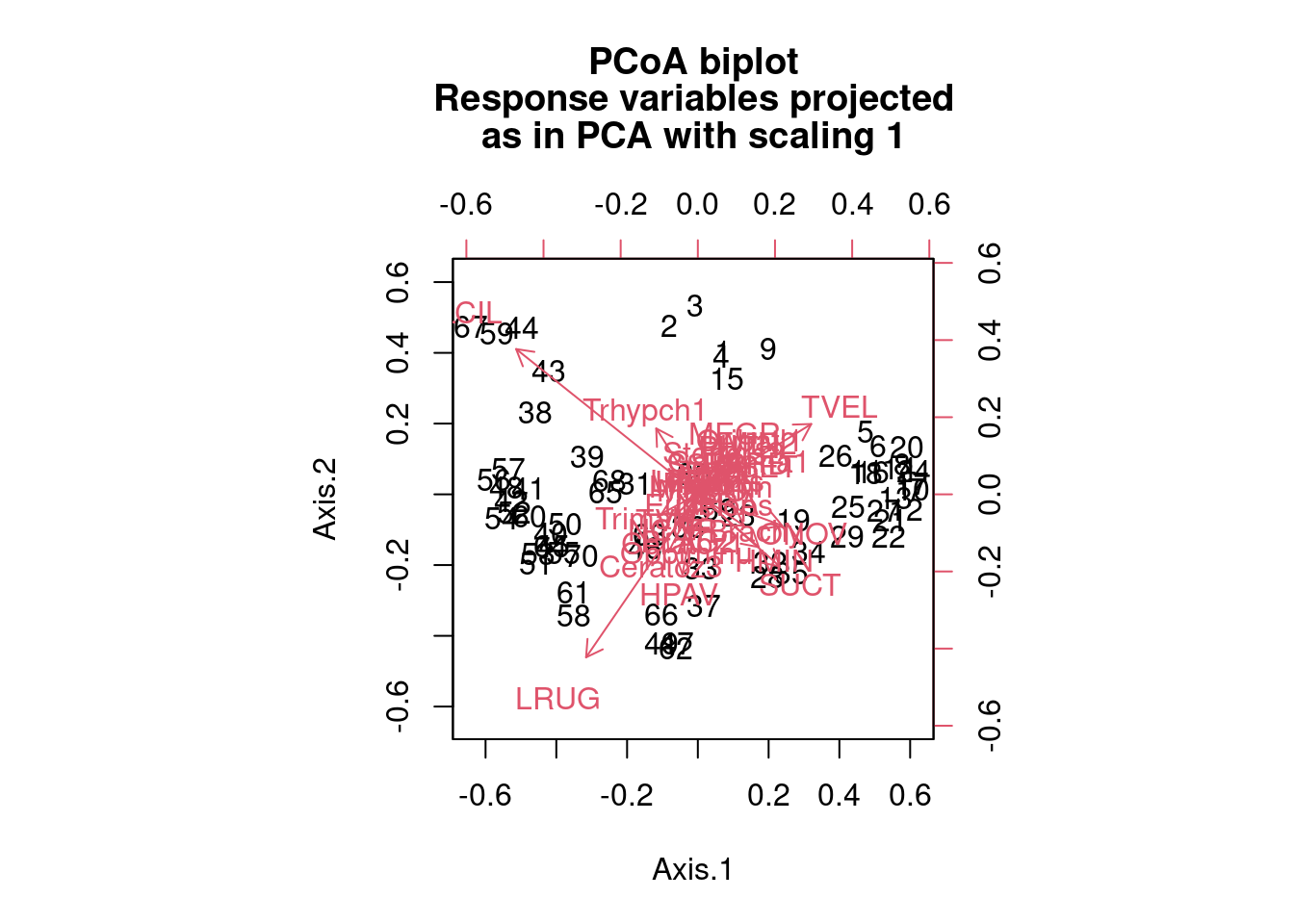

We see that species 16 and 31 are farther away from other species in terms of distance and therefore their distribution across the sites is highly dissimilar from the other species of mites (and each other). Site labels that practically overlap each other are good examples of sites with low dissimilarity (i.e. high similarity) to each other in terms of the species that are found at those sites.