Chapter 4 Example with real data

Let us use our prior knowledge on general linear models to explore the relationship between variables within the Oribatid mite data set.

Let us begin by loading this data set into R:

# Use setwd() to set your working directory

mites <- read.csv('data/mites.csv',
                  stringsAsFactors = TRUE)

The dataset that you just loaded is a subset from the classic Oribatid mites (Acari,Oribatei), which has been used in numerous texts (e.g. Borcard, Gillet & Legendre, Numerical Ecology with R), and which is available in the vegan library.

The Oribatid mite dataset has 70 observations with moss and mite samples collected at the Station de Biologie from the Université de Montréal. ], within the municipality of Saint-Hippolyte, Québec (Canada). Each sample includes 5 variables of environmental measurements and abundance for Galumna sp. for each site.

We can peek into the structure and the first six rows of the dataset using the head() and str() functions:

head(mites)

##   Galumna pa totalabund        prop SubsDens WatrCont Substrate Shrub    Topo
## 1       8  1        140 0.057142857    39.18   350.15   Sphagn1   Few Hummock
## 2       3  1        268 0.011194030    54.99   434.81    Litter   Few Hummock
## 3       1  1        186 0.005376344    46.07   371.72 Interface   Few Hummock
## 4       1  1        286 0.003496503    48.19   360.50   Sphagn1   Few Hummock
## 5       2  1        199 0.010050251    23.55   204.13   Sphagn1   Few Hummock
## 6       1  1        209 0.004784689    57.32   311.55   Sphagn1   Few Hummock

str(mites)

## 'data.frame':    70 obs. of  9 variables:
##  $ Galumna   : int  8 3 1 1 2 1 1 1 2 5 ...
##  $ pa        : int  1 1 1 1 1 1 1 1 1 1 ...
##  $ totalabund: int  140 268 186 286 199 209 162 126 123 166 ...
##  $ prop      : num  0.05714 0.01119 0.00538 0.0035 0.01005 ...
##  $ SubsDens  : num  39.2 55 46.1 48.2 23.6 ...
##  $ WatrCont  : num  350 435 372 360 204 ...
##  $ Substrate : Factor w/ 7 levels "Barepeat","Interface",..: 4 3 2 4 4 4 4 2 3 4 ...
##  $ Shrub     : Factor w/ 3 levels "Few","Many","None": 1 1 1 1 1 1 1 2 2 2 ...
##  $ Topo      : Factor w/ 2 levels "Blanket","Hummock": 2 2 2 2 2 2 2 1 1 2 ...

Our first glance into the dataset already allows us to separate potential response variables from potential predictors:

Response variables:

Occurrence: pa
Abundance: Galumna
Relative Frequency or Proportion: prop

Predictive variables:

Substract Density: SubsDens
Water Content: WatrCont
Substrate: Substrate
Shrubs Nearby: Shrub
Topography: Topo

We can also already elaborate an initial question: Could the abundance, occurrence or proportion of Galumna sp. be predicted by environmental features?

To answer this question, we can think of a variety of functions:

\(\text{Abundance} = f(\text{Water content}, \epsilon)\)

\(\text{Proportion} = f(\text{Water content}, \epsilon)\)

\(\text{Occurrence} = f(\text{Substrate}, \epsilon)\)

\(\text{Abundance} = f(\text{Topography}, \epsilon)\)

\(\text{Occurrence} = f(\text{Shrubs Nearby}, \epsilon)\)

\(\text{Relative Frequency} = f(\text{Topography}, \epsilon)\)

\(\text{Occurrence} = f(\text{Substract Density}, \epsilon)\)

\(\text{Abundance} = f(\text{Substrate}, \epsilon)\)

Can we see a relationship between Galumna and any of the five environmental variables?

Let us attempt to be more specific and ask whether he composition of Galumna’s communities (abundance, occurrence and relative frequency) vary as a function of water content?.

We can begin by representing all three response variables against the predictor:

plot(Galumna ~ WatrCont,
     data = mites,
     xlab = 'Water content',
     ylab = 'Abundance')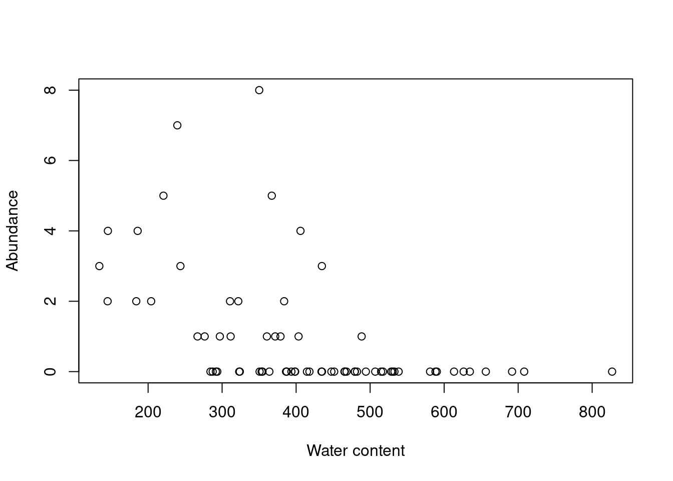

boxplot(WatrCont ~ pa,
        data = mites,
        xlab='Presence/Absence',
        ylab = 'Water content')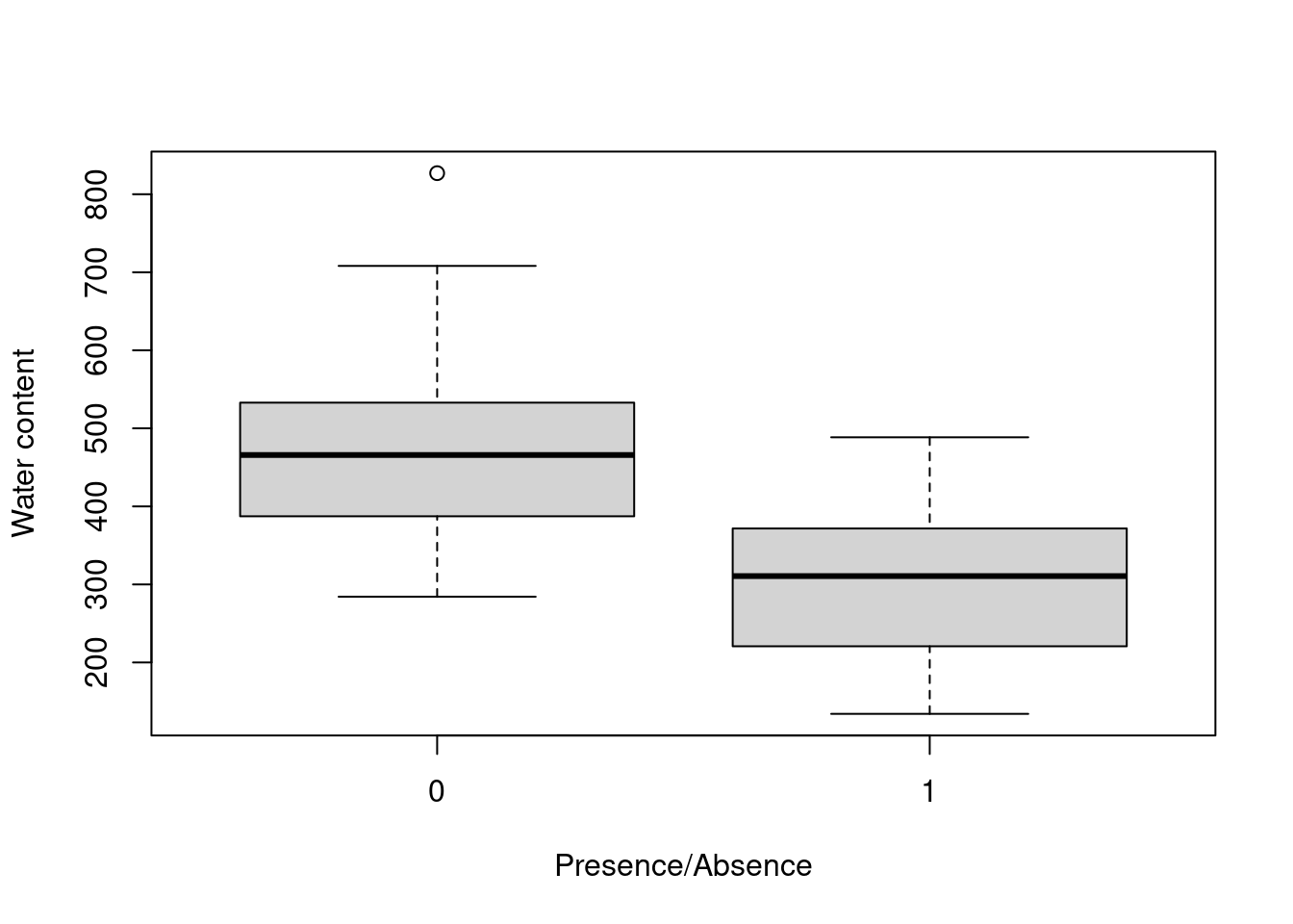

plot(prop ~ WatrCont,
     data = mites,
     xlab = 'Water content',
     ylab = 'Proportion')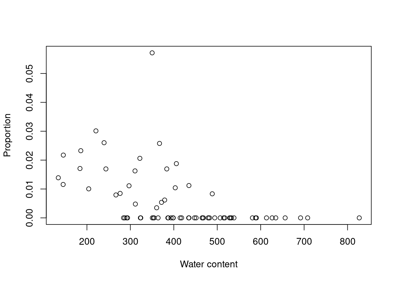

Indeed, Galumna seems to vary negatively as a function of WatrCont, i.e. Galumna sp. seems to prefer dryer sites.

We can go step further and fit general linear models to test whether Galumna, pa, or prop vary as a function of WatrCont using the lm() function:

# Fit the models
## 
# Abundance model
lm.abund <- lm(Galumna ~ WatrCont, data = mites)
## 
# Presence-absence model
lm.pa <- lm(pa ~ WatrCont, data = mites)
## 
# Proportion model
lm.prop <- lm(prop ~ WatrCont, data = mites)

Then, we can check the model output to verify whether these relationships are statistically significant:

# Check the model output with the summary() function
summary(lm.abund)

## 
## Call:
## lm(formula = Galumna ~ WatrCont, data = mites)
## 
## Residuals:
##     Min      1Q  Median      3Q     Max 
## -1.7210 -0.8236 -0.3270  0.3910  6.6772 
## 
## Coefficients:
##              Estimate Std. Error t value Pr(>|t|)    
## (Intercept)  3.439349   0.555825   6.188 3.98e-08 ***
## WatrCont    -0.006045   0.001280  -4.723 1.21e-05 ***
## ---
## Signif. codes:  0 '***' 0.001 '**' 0.01 '*' 0.05 '.' 0.1 ' ' 1
## 
## Residual standard error: 1.514 on 68 degrees of freedom
## Multiple R-squared:  0.247,  Adjusted R-squared:  0.2359 
## F-statistic: 22.31 on 1 and 68 DF,  p-value: 1.206e-05

summary(lm.pa)

## 
## Call:
## lm(formula = pa ~ WatrCont, data = mites)
## 
## Residuals:
##      Min       1Q   Median       3Q      Max 
## -0.61320 -0.30889 -0.05498  0.30247  0.80073 
## 
## Coefficients:
##               Estimate Std. Error t value Pr(>|t|)    
## (Intercept)  1.1892142  0.1431306   8.309 6.03e-12 ***
## WatrCont    -0.0020263  0.0003296  -6.148 4.68e-08 ***
## ---
## Signif. codes:  0 '***' 0.001 '**' 0.01 '*' 0.05 '.' 0.1 ' ' 1
## 
## Residual standard error: 0.3897 on 68 degrees of freedom
## Multiple R-squared:  0.3573, Adjusted R-squared:  0.3478 
## F-statistic:  37.8 on 1 and 68 DF,  p-value: 4.677e-08

summary(lm.prop)

## 
## Call:
## lm(formula = prop ~ WatrCont, data = mites)
## 
## Residuals:
##       Min        1Q    Median        3Q       Max 
## -0.010208 -0.004927 -0.002056  0.003240  0.049252 
## 
## Coefficients:
##               Estimate Std. Error t value Pr(>|t|)    
## (Intercept)  2.020e-02  3.294e-03   6.133 4.98e-08 ***
## WatrCont    -3.516e-05  7.586e-06  -4.635 1.67e-05 ***
## ---
## Signif. codes:  0 '***' 0.001 '**' 0.01 '*' 0.05 '.' 0.1 ' ' 1
## 
## Residual standard error: 0.008971 on 68 degrees of freedom
## Multiple R-squared:  0.2401, Adjusted R-squared:  0.2289 
## F-statistic: 21.49 on 1 and 68 DF,  p-value: 1.665e-05

# Extracting the Pr(>|t|)

summary(lm.abund)$coefficients[, 4]

##  (Intercept)     WatrCont 
## 3.981563e-08 1.206117e-05

summary(lm.pa)$coefficients[, 4]

##  (Intercept)     WatrCont 
## 6.030252e-12 4.676755e-08

summary(lm.prop)$coefficients[, 4]

##  (Intercept)     WatrCont 
## 4.977432e-08 1.665437e-05

For now, yes, there is a strong and significant relationship for all 3 response variables!

But, wait a minute… We are forgetting something important here!

What about the assumptions of linear models?