Chapter 15 Challenge 4

Create your own ggplot and follow these recommendations: * Dataset: any (recommended: use your dataset) * Explore a new geom_* and other plot elements (recall Chapter (ref?)/(#gg-layers))

Use the following links for tips and inspiration:

15.1 Challenge 4: Solution example 1

data(msleep)
ggplot(msleep, aes(x = vore, y = log10(brainwt), fill = vore)) +
    geom_violin() + geom_signif(comparisons = list(c("herbi",
    "insecti"))) + labs(main = "Brain weight among different vore",
    y = "log10(Brain weight (Kg))") + scale_fill_grey() + theme_classic()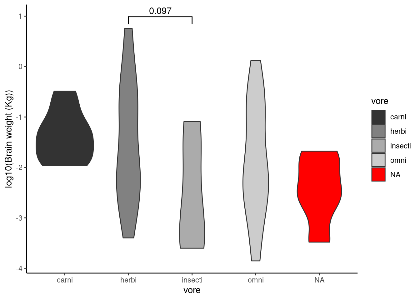

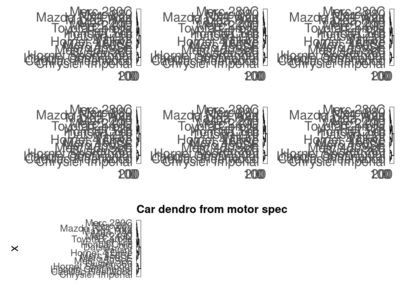
15.2 Challenge 4: Solution example 2

data(mtcars)
# let's do some clustering!
mtcars.short <- mtcars[1:20, ]
mtcars.short.hc <- hclust(dist(mtcars.short), "average")

ggdendrogram(mtcars.short.hc, rotate = TRUE) + # fine-tuning ggdendrogram(mtcars.short.hc,
ggdendrogram(mtcars.short.hc, rotate = TRUE) + # fine-tuning rotate
ggdendrogram(mtcars.short.hc, rotate = TRUE) + # fine-tuning =
ggdendrogram(mtcars.short.hc, rotate = TRUE) + # fine-tuning TRUE)
ggdendrogram(mtcars.short.hc, rotate = TRUE) + # fine-tuning +
ggdendrogram(mtcars.short.hc, rotate = TRUE) + # fine-tuning #
ggdendrogram(mtcars.short.hc, rotate = TRUE) + # fine-tuning fine-tuning
labs(title = "Car dendro from motor spec", y = "Cars") + theme(axis.title.y = element_text(size = 16),
    axis.text.y = element_text(size = 12), axis.title.x = element_blank(),
    axis.text.x = element_blank(), plot.title = element_text(size = 14,
        face = "bold"))