Workshop 2: Loading and Manipulating Data
QCBS R Workshop Series
Québec Centre for Biodiversity Science
About this workshop


Learning Objectives
1. Creating an R project
2. Writing a script
3. Loading, exploring, and saving data
4. Learn to manipulate data frames with tidyr, dplyr, and maggritr
Creating an R project
RStudio projects
- Projects make easy to keep your work organized.
- All files, scripts, and documentation related to a specific project are bound together with a .Rproj file
Encourages reproducible code!
Creating a new project
Use the New project command
(available in the global toolbar: File -> New Project)
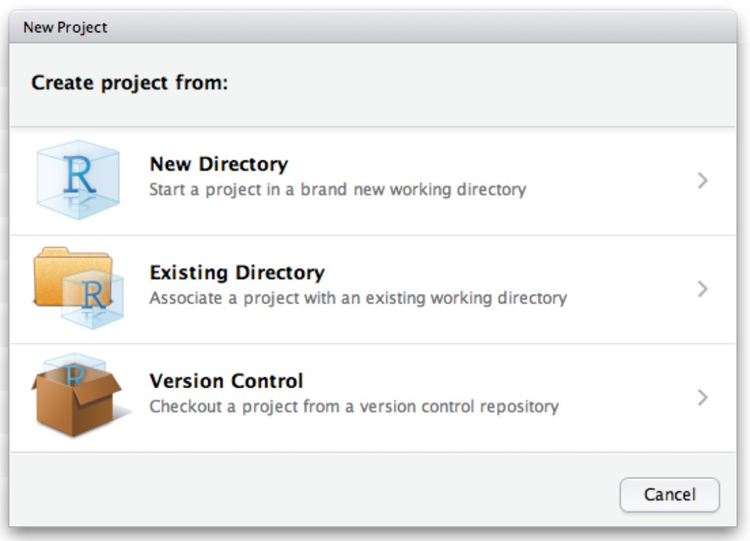
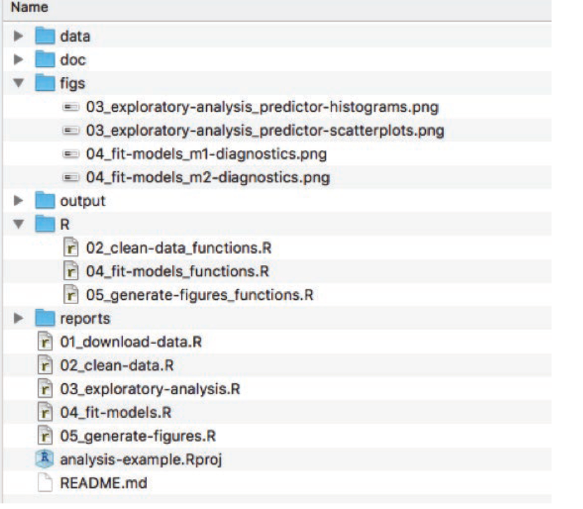
One project = one folder
Keep your files organized!
Preparing data for R
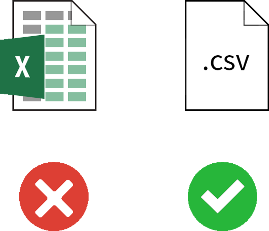
Dataset should be stored as comma-separated value files (.csv) in the working directory
- Can be created from almost all applications (Excel, LibreOffice, Google Docs)
File -> Save as .csv…
Naming files
Avoid using spaces, accents or special characters within filenames.
Recommended
rawDatasetAgo2017.csvco2_concentrations_QB.csv01_figIntro.R
Not recommended
final.csvsafnnejs.csv1-4.csv
Naming variables
Avoid using spaces, accents or special characters within variable names.
Use separators (e.g. "_") to add details
Recommended
MeasurementsspeciesNamesSite_001_Rep_002
Not recommended
a3complicatedverylongname
Check the tidyverse style guide for recommended coding habits.
Common data preparation mistakes
Here are a few examples of mistakes that originate confusion when preparing and manipulating data:
- text in numeric columns;
- typos;
- numeric names for non-numeric data;
- inconsistent formats for dates, numbers, metrics, and other units;
- incorrect headings;
- merged cells.
Read the publication by Broman & Woo (2017)
on useful tips on data organization in spreadsheets.
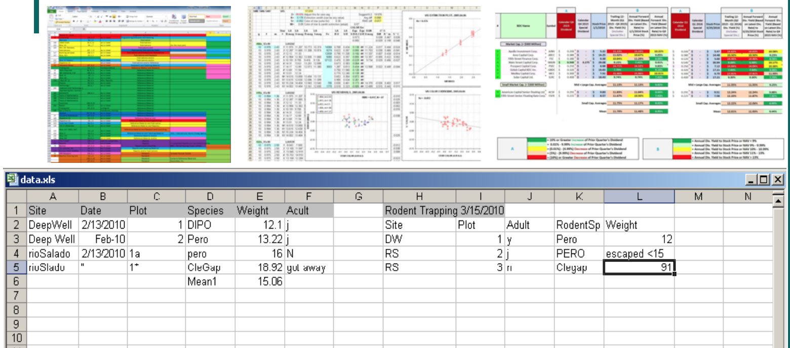
Non-recommended data tables
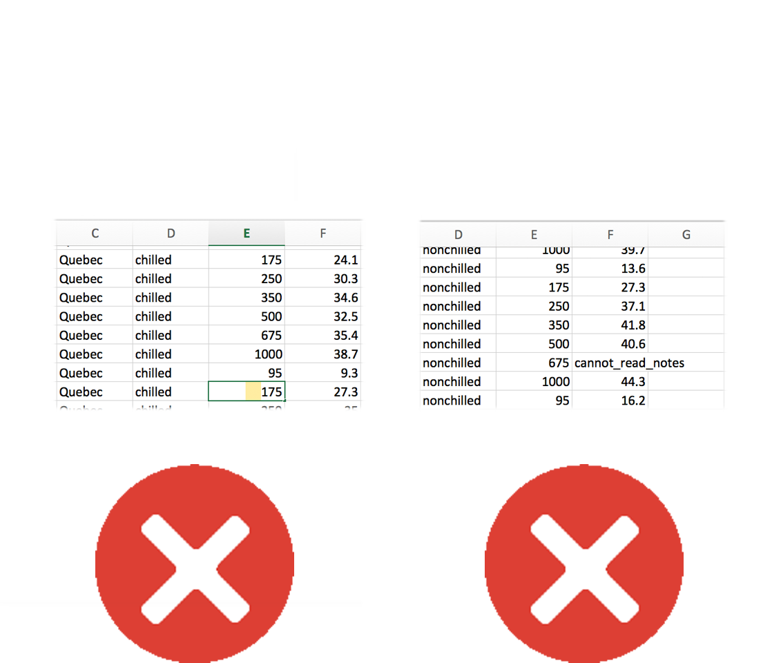
Horrible data sheets
Not the best practices for data preservation and interoperability
Preparing data in R
It is possible to prepare your data entirely within R as it:
- Saves time for large datasets;
- Keeps original data intact;
- Keeps track of the manipulation and transformation you did; and,
- Can switch between long- and wide-formats easily (more details later).
Useful tips on data preparation can be found here: https://www.zoology.ubc.ca/~schluter/R/data/
Writing a Script
R Scripts
What is a script?
- A text file storing the commands used for a particular analysis
Once written and saved, your script file allows you to make changes and re-run analyses with minimal effort!
- Just highlight text and click "Run" or press
Command + Enter(Apple) orCtrl + Enter/Ctrl + R(Windows and Linux)
- Just highlight text and click "Run" or press
Creating an R script
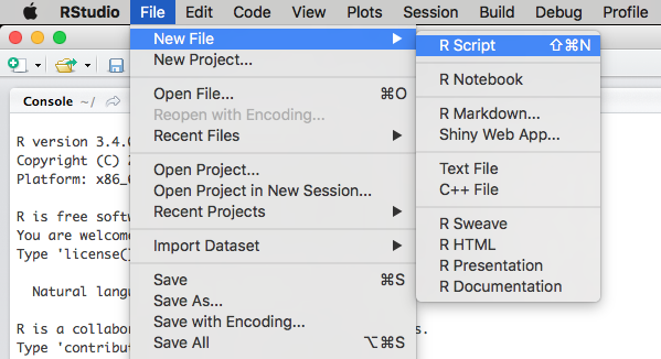
Creating an R script
![]()
Commands and comments
The # symbol in a script tells R to not run and ignore anything written past it within the same line
a <- 1 + 1# This is a commentb <- 2 + 2 # This is a commentWhy should I use #?
- Annotating someone’s script is a good way to learn;
- Tell collaborators what you did;
- Good step towards reproducible science.
Be as detailed as possible!
Header
It is recommended that you start your script with a header using comments:
![]()
Section Headings
You can make a section heading in R Studio with four # signs
# You can comment using this. # Look below how to create section headers:#### Heading name ##### You can also do this:# Section One ---------------------------------# Section Two =================================### Section Three #############################Section Headings
This allows you to move quickly between sections and hide sections
![]()
Preparing your R Environment: Housekeeping
The first command at the top of all scripts may be: rm(list = ls()).
This command:
- Clears objects from the memory and the disk;
- Prevents errors related to the use of out-dated data.
# Clear the R Workspacerm(list = ls())?rm?lsPreparing your R Environment: Housekeeping
DIY: Try adding some test data to R and then see how rm(list = ls()) removes it
A<-"Test" # Put some data in workspaceA <- "Test" # Add some spaces to organize your data!A = "Test" # You can do this, but it does not mean you should# Check objects in the workspacels()# [1] "A"A# [1] "Test"# Clean Workspacerm(list=ls())A# Error in eval(expr, envir, enclos): object 'A' not foundRemember
Ris ready for commands when you see the chevron>in the console. If you do not see it, pressEsc
Ris case sensitive!
Loading, exploring and saving data
Download today's data
You can download the data for this workshop here:
https://github.com/QCBSRworkshops/workshop02/tree/main/pres-en/data
And the script here:
https://r.qcbs.ca/workshop02/book-en/workshop02-script-en.R
Save the files in the folder where your created your R project.
Download today's data
You can download the data for this workshop here:
https://github.com/QCBSRworkshops/workshop02/tree/main/pres-en/data
And the script here:
https://r.qcbs.ca/workshop02/book-en/workshop02-script-en.R
Save the files in the folder where your created your R project.
NOTE Many databases are already available within R
# Complete list of available data on base Rlibrary(help = "datasets")Working Directory
If you are not using an RStudio project, you have to tell R where your scripts and data are.Type getwd() in the console to see your current working directory:
getwd()If you want to change your working directory use setwd():
setwd("C:/Users/my_new_path")It is recommended to create an RStudio project and avoid using setwd() to promote reproducibility
Display contents of the directory
You can display contents of the working directory using dir():
dir()# [1] "assets" "data" # [3] "images" "qcbsR-fonts.css" # [5] "qcbsR-header.html" "qcbsR-macros.js" # [7] "qcbsR.css" "workshop02-en.Rproj" # [9] "workshop02-pres-en_cache" "workshop02-pres-en.Rmd"It helps to:
- Check that the file you plan to open is present in the folder that R is currently working in
- Check for correct spelling (e.g.
co2_good.csvinstead ofCO2_good.csv)
Importing Data
Import data into R using read.csv():
CO2 <- read.csv("data/co2_good.csv", header=TRUE)Note that this will:
- Create a new object in R called
CO2; - The file name is written within quotation marks ('file' or "file");
- If you needed to fetch the file name from another directory that is not yours, you would have to write the full extension (e.g.,
"C:/Users/Mario/Downloads/co2_good.csv") header=TRUEtells R that the first line of your dataset contains column names
Importing Data
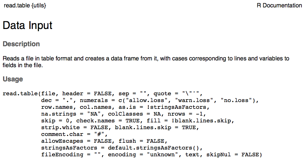
Recall to find out what arguments the function requires, use help “?”
I
?read.csvNote that if your operating system or CSV editor (e.g. Excel) is in French, you may have to use read.csv2()
?read.csv2Importing Data
![]()
Notice that RStudio now provides information on the CO2 data in your workspace.
The workspace refers to all the objects that you create during an R session.
Inspecting the data
| R Command | Action |
|---|---|
CO2 |
look at the whole dataframe |
view(CO2) |
look data as a spreadsheet |
head(CO2) |
look at the first few rows |
tail(CO2) |
look at the last few rows |
names(CO2) |
names of the columns in the dataframe |
attributes(CO2) |
attributes of the dataframe |
dim(CO2) |
dimensions of the dataframe |
ncol(CO2) |
number of columns |
nrow(CO2) |
number of rows |
summary(CO2) |
basic statistics for each variables |
NOTE These functions could also be used with other objects such as vector, matrix, list, array, etc.
Inspecting the data
str(CO2)# 'data.frame': 84 obs. of 5 variables:# $ Plant : chr "Qn1" "Qn1" "Qn1" "Qn1" ...# $ Type : chr "Quebec" "Quebec" "Quebec" "Quebec" ...# $ Treatment: chr "nonchilled" "nonchilled" "nonchilled" "nonchilled" ...# $ conc : int 95 175 250 350 500 675 1000 95 175 250 ...# $ uptake : num 16 30.4 34.8 37.2 35.3 39.2 39.7 13.6 27.3 37.1 ...This shows the structure of the dataframe. Very useful to check data type (mode) of all columns to make sure R loaded data properly.
Note: the CO2 dataset includes repeated measurements of CO2 uptake from 6 plants from Quebec and 6 plants from Mississippi at several levels of CO2 concentration. Half the plants of each type were chilled overnight before the experiment was conducted.
Inspecting the data
Common problems:
- Factors loaded as text (character) or viceversa
- Factors includes too many (and unexpected) levels because of typos
- Data (integer or numeric) is loaded as character because of typos (e.g. a space or a "," instead of a "." to separate decimal numbers)
Exercise
Load the data with:
CO2 <- read.csv("data/co2_good.csv", header = FALSE)Check data types with str() again.
What is wrong here?
Exercise
Load the data with:
CO2 <- read.csv("data/co2_good.csv", header = FALSE)Check data types with str() again.
What is wrong here?
Do not forget to re-load data with header = TRUE afterwards
Reminder from Workshop 1: Accessing data
Imagine a data frame called mydata:
mydata[2,3] # Extracts the content of row 2 / column 3mydata[1,] # Extracts the first rowmydata[,1] # Extracts the first columnmydata[,1][2] # [...] can be also be used recursivelymydata$Variable1 # Also extracts the first columnRenaming variables
Variables names can be changed within R.
# First lets make a copy of the dataset to play withCO2copy <- CO2# names() gives you the names of# the variables present in the data framenames(CO2copy)# [1] "Plant" "Type" "Treatment" "conc" "uptake"# Changing from English to French names # (make sure you have the same levels!)names(CO2copy) <- c("Plante","Categorie", "Traitement", "conc", "absortion")names(CO2copy)# [1] "Plante" "Categorie" "Traitement" "conc" "absortion"Creating new variables
Variables and strings can be concatenated together.
The function paste() is very useful for concatenating.
See ?paste and ?paste0.
# Let us create an unique id for our samples:# Do not forget to use "" for stringsCO2copy$uniqueID <- paste0(CO2copy$Plante, "_",CO2copy$Categorie, "_", CO2copy$Traitement)# observe the resultshead(CO2copy$uniqueID)# [1] "Qn1_Quebec_nonchilled" "Qn1_Quebec_nonchilled" "Qn1_Quebec_nonchilled"# [4] "Qn1_Quebec_nonchilled" "Qn1_Quebec_nonchilled" "Qn1_Quebec_nonchilled"Creating new variables
Creating new variables works for numbers and mathematical operations as well!
# Let us standardize our variable "absortion" to relative valuesCO2copy$absortionRel <- CO2copy$absortion/max(CO2copy$absortion)# Observe the resultshead(CO2copy$absortionRel)Subsetting data
There are many ways to subset a data frame
# Let us keep working with our CO2copy data frame# Select only "Plante" and "absortionRel" columns.# (Do not forget the ","!)CO2copy[,c("Plante", "absortionRel")]# Subset data frame from rows from 1 to 50CO2copy[1:50,]Subsetting data
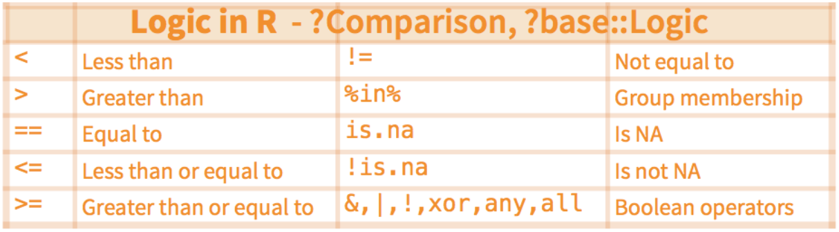
# Select observations matching only the nonchilled Traitement.CO2copy[CO2copy$Traitement == "nonchilled",]# Select observations with absortion # higher or equal to 20CO2copy[CO2copy$absortion >= 20, ]# Select observations with absortion # higher or equal to 20CO2copy[CO2copy$Traitement == "nonchilled" & CO2copy$absortion >= 20, ]# We are done playing with the Dataset copy, lets erase it.rm(CO2copy)Go here to check all the logical operators you can use
Data exploration
A good way to start your data exploration is to look at some basic statistics of your dataset.
Use the summary() function to do that!
summary(CO2)This is also useful to spot some errors you might have missed!
Data exploration
You can also use other functions to calculate basic statistics on parts of your data frame. Let us try the mean(), sd() and hist() functions:
# Calculate the mean and the standard deviation # of the CO2 concentration:# Assign them to new variablesmeanConc <- mean(CO2$conc)sdConc <- sd(CO2$conc)# print() prints any given value to the R consoleprint(paste("the mean of concentration is:", meanConc))# [1] "the mean of concentration is: 435"print(paste("the standard deviation of concentration is:", sdConc))# [1] "the standard deviation of concentration is: 295.924119222056"Data exploration
# Let us plot a histogram to explore the distribution of "uptake"hist(CO2$uptake)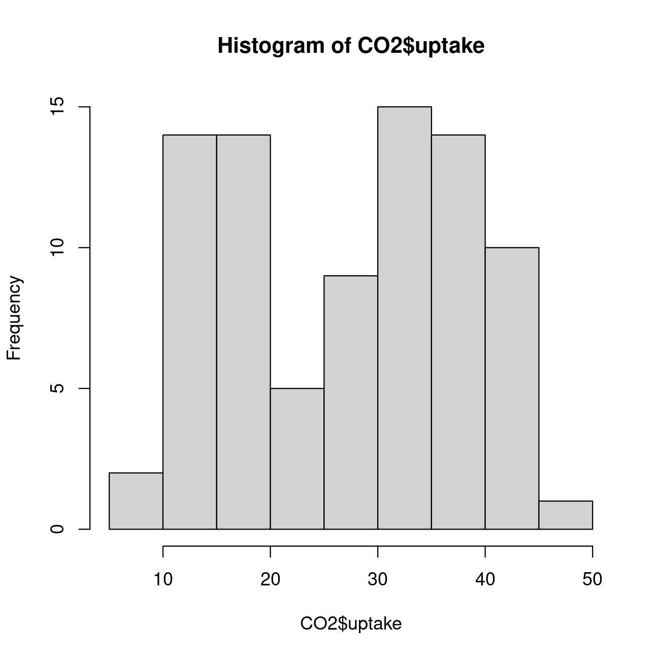
Data exploration
# Increasing the number of bins to observe better the patternhist(CO2$uptake, breaks = 40)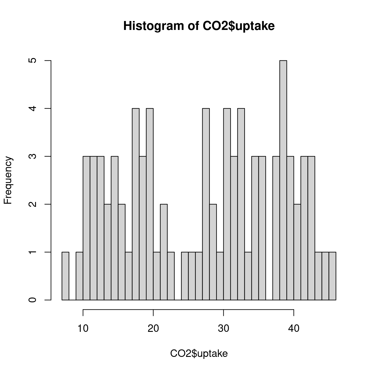
The apply() function
The function apply() can be used to apply a function to multiple
columns of your data simultaneously. Use the ?apply command to get
more information about apply().
?applyTo use apply, you have to specify three arguments. The first argument is the data you would like to apply the function to; the second argument is whether you would like to calculate based on rows (1) or columns (2) of your dataset; the third argument is the function you would like to apply. For example:
# Calculate mean of the two columns in the data frame that contain continuous dataapply(CO2[,4:5], MARGIN = 2, FUN = mean)Saving your Workspace
# Saving an R workspace file that stores all your objectssave.image(file="data/co2_project_Data.RData")# Clear your memoryrm(list = ls())# Reload your dataload("data/co2_project_Data.RData")head(CO2) # Looking good!# Plant Type Treatment conc uptake# 1 Qn1 Quebec nonchilled 95 16.0# 2 Qn1 Quebec nonchilled 175 30.4# 3 Qn1 Quebec nonchilled 250 34.8# 4 Qn1 Quebec nonchilled 350 37.2# 5 Qn1 Quebec nonchilled 500 35.3# 6 Qn1 Quebec nonchilled 675 39.2Exporting data
R disposes of write functions that allow you to write objects directly to files in your computer. Let us use the write.csv() function to save our CO2 data into a .CSV file:
write.csv(CO2, file = "data/co2_new.csv")Note that our arguments are both:
CO2 Object (name)
"co2_new.csv" File to write (name)
Challenge: Use your data 
- Try to load, explore, plot, and save your own data in R;
- If it does not load properly, try to make the appropriate changes;
- When you are finished, try opening your exported data in Excel, Numbers, Notepad or TextEdit.
If you don’t have your own data, work with your neighbor
Remember to clean your workspace
Database repair
Database repair
Getting your data working properly can be tougher than you think!
For example, sharing data from an Apple computer to Windows, or between computers set up in different continents can lead to incompatible files (e.g. different decimal separators).
Let us practice how to solve these common errors.
Database repair
Exercise:
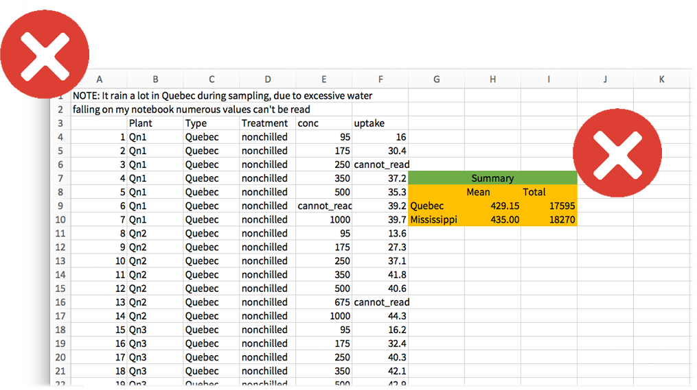
Read the file co2_broken.csv
CO2 <- read.csv("data/co2_broken.csv")head(CO2)# NOTE..It.rain.a.lot.in.Quebec.during.sampling due.to.excessive X# 1 falling on my notebook numerous values can't be read rain NA NA# 2 Plant\tType\tTreatment\tconc\tuptake NA NA# 3 Qn1\tQuebec\tnonchilled\t95\t16 NA NA# 4 Qn1\tQuebec\tnonchilled\t175\t30.4 NA NA# 5 Qn1\tQuebec\tnonchilled\t250\tcannot_read_notes NA NA# 6 Qn1\tQuebec\tnonchilled\t350\t37.2 NA NA# X.1 X.2 X.3# 1 NA NA NA# 2 NA NA NA# 3 NA NA NA# 4 NA NA NA# 5 NA NA NA# 6 NA NA NADatabase repair
Some useful functions:
head()- first few rowsstr()- structure of dataclass()- class of the objectunique()- unique observationslevels()- levels of a factorwhich()- ask a question to your data framedroplevels()- get rid of undesired levels after sub setting factors
add "?" (e.g. ?read.csv to the function name to access the function help page)
HINT There are 4 problems!
Database repair
ERROR 1 The data appears to be lumped into one column
head(CO2)# NOTE..It.rain.a.lot.in.Quebec.during.sampling due.to.excessive X# 1 falling on my notebook numerous values can't be read rain NA NA# 2 Plant\tType\tTreatment\tconc\tuptake NA NA# 3 Qn1\tQuebec\tnonchilled\t95\t16 NA NA# 4 Qn1\tQuebec\tnonchilled\t175\t30.4 NA NA# 5 Qn1\tQuebec\tnonchilled\t250\tcannot_read_notes NA NA# 6 Qn1\tQuebec\tnonchilled\t350\t37.2 NA NA# X.1 X.2 X.3# 1 NA NA NA# 2 NA NA NA# 3 NA NA NA# 4 NA NA NA# 5 NA NA NA# 6 NA NA NADatabase repair
ERROR 1 - Solution
- Re-import the data, but specify the separation among entries
- The sep argument tells R what character separates the values on each line of the file
- Here, "TAB" was used instead of ","
CO2 <- read.csv("data/co2_broken.csv",sep = "")Database repair
ERROR 2 The data does not start until the third line of the file, so you end up with notes on the file as the headings.
head(CO2)# NOTE. It rain a lot in. Quebec during# 1 falling on my notebook numerous values can't be# 2 Plant Type Treatment conc uptake # 3 Qn1 Quebec nonchilled 95 16 # 4 Qn1 Quebec nonchilled 175 30.4 # 5 Qn1 Quebec nonchilled 250 cannot_read_notes # 6 Qn1 Quebec nonchilled 350 37.2 # sampling. due to excessive X....# 1 read rain,,,, NA NA NA# 2 NA NA NA# 3 NA NA NA# 4 NA NA NA# 5 NA NA NA# 6 NA NA NADatabase repair
ERROR 2 - Solution
Skip two lines when loading the file using the "skip" argument:
CO2 <- read.csv("data/co2_broken.csv", sep = "", skip = 2)head(CO2)# Plant Type Treatment conc uptake# 1 Qn1 Quebec nonchilled 95 16# 2 Qn1 Quebec nonchilled 175 30.4# 3 Qn1 Quebec nonchilled 250 cannot_read_notes# 4 Qn1 Quebec nonchilled 350 37.2# 5 Qn1 Quebec nonchilled 500 35.3# 6 Qn1 Quebec nonchilled cannot_read_notes 39.2Database repair
ERROR 3 conc and uptake variables are considered factors instead of numbers, because there are comments in the numeric columns
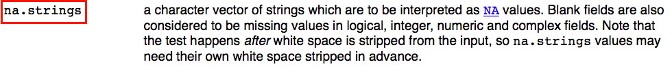
str(CO2)# 'data.frame': 84 obs. of 5 variables:# $ Plant : chr "Qn1" "Qn1" "Qn1" "Qn1" ...# $ Type : chr "Quebec" "Quebec" "Quebec" "Quebec" ...# $ Treatment: chr "nonchilled" "nonchilled" "nonchilled" "nonchilled" ...# $ conc : chr "95" "175" "250" "350" ...# $ uptake : chr "16" "30.4" "cannot_read_notes" "37.2" ...unique(CO2$conc)# [1] "95" "175" "250" # [4] "350" "500" "cannot_read_notes"# [7] "1000" "675"- Due to missing values entered as "cannot_read_notes" and "na"
- Recall that R only recognizes "NA" (capital)
?read.csv
Database repair
ERROR 3 - Solution
Tell R that all of NA, "na", and "cannot_read_notes" should be considered NA. Then because all other values in those columns are numbers, conc and uptake will be loaded as numeric/integer.
CO2 <- read.csv("data/co2_broken.csv", sep = "", skip = 2, na.strings = c("NA","na", "cannot_read_notes"))str(CO2)# 'data.frame': 84 obs. of 5 variables:# $ Plant : chr "Qn1" "Qn1" "Qn1" "Qn1" ...# $ Type : chr "Quebec" "Quebec" "Quebec" "Quebec" ...# $ Treatment: chr "nonchilled" "nonchilled" "nonchilled" "nonchilled" ...# $ conc : int 95 175 250 350 500 NA 1000 95 175 250 ...# $ uptake : num 16 30.4 NA 37.2 35.3 39.2 39.7 13.6 27.3 37.1 ...Database repair
ERROR 4
There are only 2 treatments (chilled and non-chilled) but there are spelling errors causing it to look like 4 different treatments.
str(CO2)levels(CO2$Treatment)# NULLunique(CO2$Treatment)# [1] "nonchilled" "nnchilled" "chilled" "chiled"Database repair
ERROR 4 - Solution
# Identify all rows that contain "nnchilled" # and replace with "nonchilled"CO2$Treatment[CO2$Treatment=="nnchilled"] <- "nonchilled"# Identify all rows that contain "chiled" # and replace with "chilled"CO2$Treatment[CO2$Treatment=="chiled"] <- "chilled"Database repair
ERROR 4 - Solution
After repairing the factors, we need to remove the unused factor levels
If not :
boxplot(uptake ~ Treatment, data = CO2)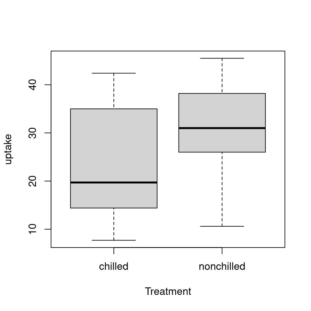
Database repair
ERROR 4 - Solution
CO2 <- droplevels(CO2)str(CO2)# 'data.frame': 84 obs. of 5 variables:# $ Plant : chr "Qn1" "Qn1" "Qn1" "Qn1" ...# $ Type : chr "Quebec" "Quebec" "Quebec" "Quebec" ...# $ Treatment: chr "nonchilled" "nonchilled" "nonchilled" "nonchilled" ...# $ conc : int 95 175 250 350 500 NA 1000 95 175 250 ...# $ uptake : num 16 30.4 NA 37.2 35.3 39.2 39.7 13.6 27.3 37.1 ...Database repair
boxplot(uptake ~ Treatment, data = CO2)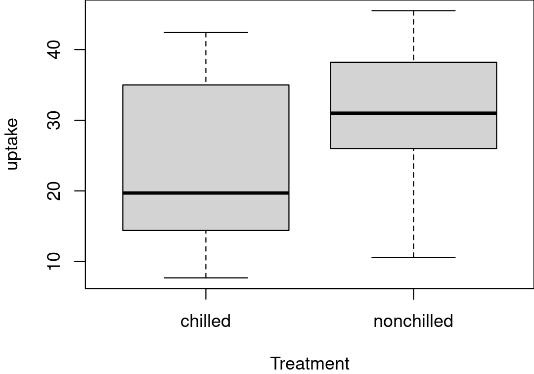
Welcome to the tidyverse world!
What is Tidyverse?
Tidyverse is a collection of packages designed for data science.
Tidyverse provides more efficient and user-friendly tools that you are likely to use in everyday data analyses.
All packages included in tidyverse are automatically installed when installing the tidyverse package: install.packages("tidyverse")
Tidyverse includes:
tidyr: tidy datadplyr: data manipulationmaggritr: provide piping operatorsggplot2: make graphicsreadr: read data (faster!)lubridate: manipulate data-time data- and more!
Learn to manipulate data with
tidyr, dyplr, and maggritr
Using tidyr to reshape data frames
library(tidyr)Data formats
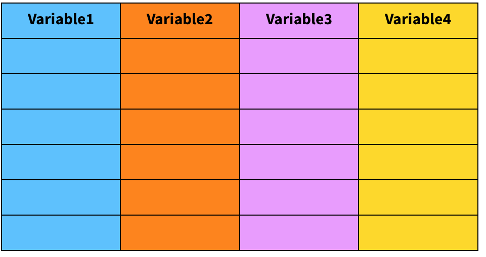
Wide format
Data format has a separate column for each variable or each factor in your study
# Species DBH Height# 1 Oak 12 56# 2 Elm 20 85# 3 Ash 13 55Long format
Data format has a column for possible variables and a column for the values of those variables
# # A tibble: 6 × 3# Species name value# <chr> <chr> <dbl># 1 Oak DBH 12# 2 Oak Height 56# 3 Elm DBH 20# 4 Elm Height 85# 5 Ash DBH 13# 6 Ash Height 55Wide data frame can be used for some basic plotting in ggplot2, but more complex plots require long format (example to come)
dplyr, lm(), glm(), gam() all require long data format
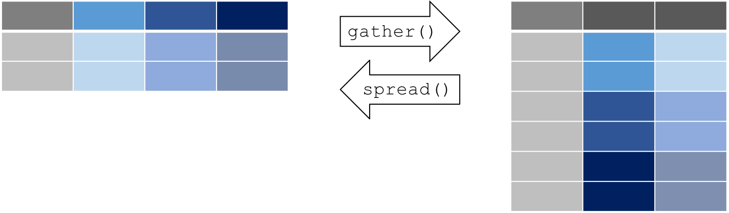
Tidying your data
Tidying allows you to manipulate the structure of your data while preserving all original information
pivot_longer() - convert from wide to long format (gather)
pivot_wider() - convert from long to wide format (spread)
tidyr installation
install.packages("tidyr")library(tidyr)Gather columns into rows
pivot_longer(data, cols, names_to, values_to, ...)
dataA data frame (e.g.wide)colsname or numeric index of the columns we wish to gather (e.g.DBH,Height)names_toname of the new column containing variable names (e.g.Dimension)values_toname of the new column containing variable values (e.g.cm)
Example of pivot_longer
wide <- data.frame(Species = c("Oak", "Elm", "Ash"), DBH = c(12, 20, 13), Height = c(56, 85, 55))wide# Species DBH Height# 1 Oak 12 56# 2 Elm 20 85# 3 Ash 13 55long <- pivot_longer(data = wide, cols = c("DBH", "Height"), names_to = "dimension", values_to = "cm")long# # A tibble: 6 × 3# Species dimension cm# <chr> <chr> <dbl># 1 Oak DBH 12# 2 Oak Height 56# 3 Elm DBH 20# 4 Elm Height 85# 5 Ash DBH 13# 6 Ash Height 55Spread rows into columns
pivot_wider(data, names_from, values_from, ...)
dataA data frame (e.g.long)names_fromname of the column containing the variable names (e.g.dimension)values_fromname of the column containing variable values (e.g.cm)
Disperser avec pivot_wider()
long# # A tibble: 6 × 3# Species dimension cm# <chr> <chr> <dbl># 1 Oak DBH 12# 2 Oak Height 56# 3 Elm DBH 20# 4 Elm Height 85# 5 Ash DBH 13# 6 Ash Height 55large2 <- pivot_wider(data = long, names_from = "dimension", values_from = "cm")large2# # A tibble: 3 × 3# Species DBH Height# <chr> <dbl> <dbl># 1 Oak 12 56# 2 Elm 20 85# 3 Ash 13 55A tibble structure for your data
Tibble is an alternate, more convenient, version for a data frame. Using tibble ensures good coding practices that can be missed using data.frame. For instance, it does not change the type of inputs (e.g. string to factors).
tibble(x = 1:3, y = c("a","b","c"))# # A tibble: 3 × 2# x y # <int> <chr># 1 1 a # 2 2 b # 3 3 cA tibble structure for your data
In addition, tibble simplifies the use of nested lists.
Example:
tibble(x = 1:3, y = list(1:5, 1:10, 1:20))# # A tibble: 3 × 2# x y # <int> <list> # 1 1 <int [5]> # 2 2 <int [10]># 3 3 <int [20]>You can use with a tibble all the functions applied to a data.frame.
separate columns
separate() splits a columns by a character string separator

separate(data, col, into, sep)
dataA data frame (e.g.long)colName of the column you wish to separateintoNames of new variables to createsepCharacter which indicates where to separate
Using separate() example
Create a fictional dataset about fish and plankton
set.seed(8)messy <- data.frame(id = 1:4, trt = sample(rep(c('control', 'farm'), each = 2)), zooplankton.T1 = runif(4), fish.T1 = runif(4), zooplankton.T2 = runif(4), fish.T2 = runif(4))messy# id trt zooplankton.T1 fish.T1 zooplankton.T2 fish.T2# 1 1 farm 0.7189275 0.64449114 0.544962116 0.2644589# 2 2 farm 0.2908734 0.45704489 0.138224346 0.2765322# 3 3 control 0.9322698 0.08930101 0.927812252 0.5211070# 4 4 control 0.7691470 0.43239137 0.001301721 0.2236889Using separate() example
First convert the messy data frame from wide to long format
messy.long <- pivot_longer(messy, names_to = "taxa", cols = c("zooplankton.T1", "fish.T1", "zooplankton.T2", "fish.T2"))head(messy.long)# # A tibble: 6 × 4# id trt taxa value# <int> <chr> <chr> <dbl># 1 1 farm zooplankton.T1 0.719# 2 1 farm fish.T1 0.644# 3 1 farm zooplankton.T2 0.545# 4 1 farm fish.T2 0.264# 5 2 farm zooplankton.T1 0.291# 6 2 farm fish.T1 0.457Using separate() example
Then we want to split the 2 sampling time (T1 and T2).
messy.long.sep <- separate(messy.long, taxa, into = c("species", "time"), sep = "\\.")head(messy.long.sep)# # A tibble: 6 × 5# id trt species time value# <int> <chr> <chr> <chr> <dbl># 1 1 farm zooplankton T1 0.719# 2 1 farm fish T1 0.644# 3 1 farm zooplankton T2 0.545# 4 1 farm fish T2 0.264# 5 2 farm zooplankton T1 0.291# 6 2 farm fish T1 0.457Recap of tidyr
A package that reshapes the layout of data sets.
Converting from wide to long format using pivot_longer()
Converting from long format to wide format using pivot_wider()
Split and merge columns with unite() and separate()
Data Wrangling with dplyr and tidyr Cheat Sheet
Challenge #1
Using the airquality dataset, gather all the columns (except Month and Day) into rows.
?airqualitydata(airquality)Solution #1
Using the airquality dataset, gather all the columns (except Month and Day) into rows.
air.long <- pivot_longer(airquality, cols = c("Ozone", "Solar.R", "Wind", "Temp"), names_to = c("variable") )head(air.long)# # A tibble: 6 × 4# Month Day variable value# <int> <int> <chr> <dbl># 1 5 1 Ozone 41 # 2 5 1 Solar.R 190 # 3 5 1 Wind 7.4# 4 5 1 Temp 67 # 5 5 2 Ozone 36 # 6 5 2 Solar.R 118Challenge #2
Spread the resulting data frame to return to the original data format.
Solution #2
Spread the resulting data frame to return to the original data format.
air.wide <- pivot_wider(air.long, values_from = "value", names_from = "variable")head(air.wide)# # A tibble: 6 × 6# Month Day Ozone Solar.R Wind Temp# <int> <int> <dbl> <dbl> <dbl> <dbl># 1 5 1 41 190 7.4 67# 2 5 2 36 118 8 72# 3 5 3 12 149 12.6 74# 4 5 4 18 313 11.5 62# 5 5 5 NA NA 14.3 56# 6 5 6 28 NA 14.9 66Data manipulation with dplyr
Intro to dplyr
- Package that contains a set of functions (or “verbs”) for data manipulation such as filtering rows, selecting specific columns, re-ordering rows, adding new columns and summarizing data;
- Easy and intuitive functions
- Fast and efficient
- Can interface with external databases and translate your R code into SQL queries
Some corresponding R base functions:
split(), subset(), apply(), sapply(), lapply(), tapply() and aggregate()
Intro to dplyr
library(dplyr)Basic functions in dplyr
These 4 core functions tackle the most common manipulations when working with data frames
select(): select columns from a data framefilter(): filter rows according to defined criteriaarrange(): re-order data based on criteria (e.g. ascending, descending)mutate(): create or transform values in a column
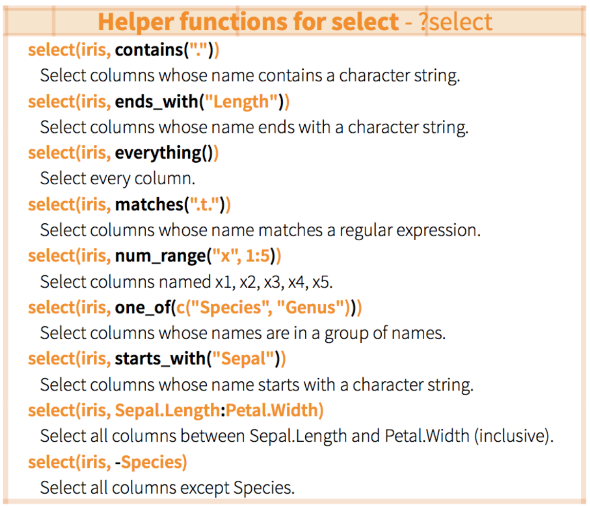
select() columns
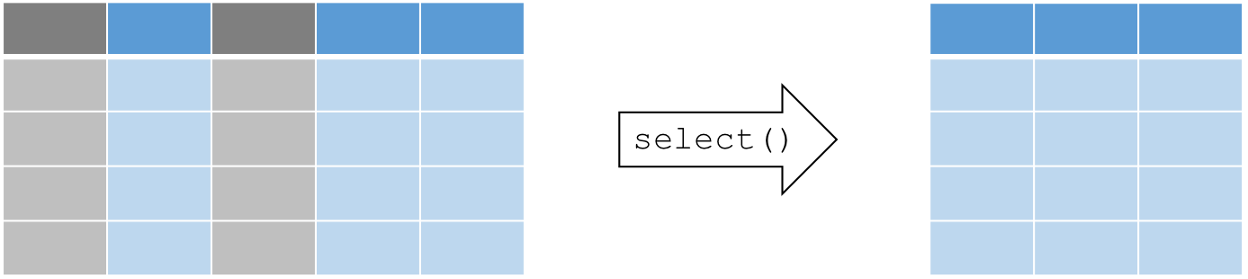
select(data, ...)
...Can be column names or positions or complex expressions separated by commas
Examples:
select(data, column1, column2) # select columns 1 and 2select(data, c(2:4,6)) # select columns 2 to 4 and 6select(data, -column1) # select all columns except column 1select(data, start_with(x.)) # select all columns that start with "x."select() columns
select() columns
Example: suppose we are only interested in the variation of Ozone over time within the airquality dataset
ozone <- select(airquality, Ozone, Month, Day)head(ozone)# Ozone Month Day# 1 41 5 1# 2 36 5 2# 3 12 5 3# 4 18 5 4# 5 NA 5 5# 6 28 5 6filter() rows
Extract a subset of rows that meet one or more specific conditions
filter(dataframe, logical statement 1, logical statement 2, ...)
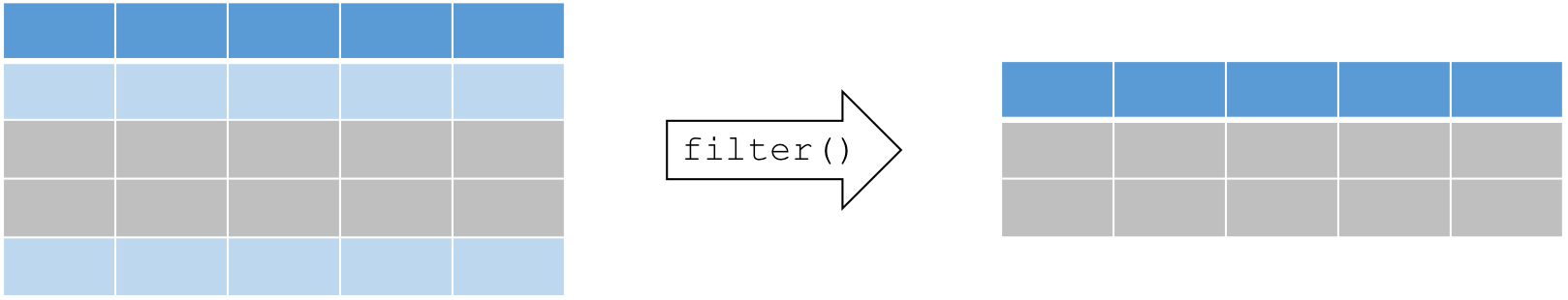
filter() rows
Example: we are interested in analyses that focus on the month of August during high temperature events
august <- filter(airquality, Month == 8, Temp >= 90)# same as: filter(airquality, Month == 8 & Temp >= 90)head(august)# Ozone Solar.R Wind Temp Month Day# 1 89 229 10.3 90 8 8# 2 110 207 8.0 90 8 9# 3 NA 222 8.6 92 8 10# 4 76 203 9.7 97 8 28# 5 118 225 2.3 94 8 29# 6 84 237 6.3 96 8 30Sort rows with arrange
Re-order rows by a particular column, by default in ascending order
Use desc() for descending order.
arrange(data, variable1, desc(variable2), ...)
Sort rows with arrange()
Example:
- Let us use the following code to create a scrambled version of the airquality dataset
air_mess <- sample_frac(airquality, 1)head(air_mess)# Ozone Solar.R Wind Temp Month Day# 1 23 115 7.4 76 8 18# 2 28 273 11.5 82 8 13# 3 8 19 20.1 61 5 9# 4 135 269 4.1 84 7 1# 5 23 299 8.6 65 5 7# 6 30 322 11.5 68 5 19Sort rows with arrange()
Example:
- Now let us arrange the data frame back into chronological order, sorting by Month then Day
air_chron <- arrange(air_mess, Month, Day)head(air_chron)# Ozone Solar.R Wind Temp Month Day# 1 41 190 7.4 67 5 1# 2 36 118 8.0 72 5 2# 3 12 149 12.6 74 5 3# 4 18 313 11.5 62 5 4# 5 NA NA 14.3 56 5 5# 6 28 NA 14.9 66 5 6Try : arrange(air_mess, Day, Month) and see the difference.
Create new columns using mutate()
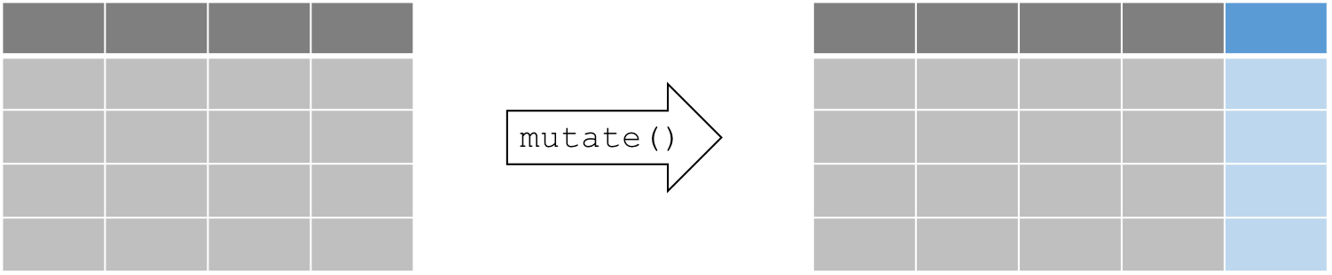
Compute and add new columns
mutate(data, newVar1 = expression1, newVar2 = expression2, ...)
Create new columns using mutate()
Example: we want to convert the temperature variable form degrees Fahrenheit to degrees Celsius
airquality_C <- mutate(airquality, Temp_C = (Temp-32)*(5/9))head(airquality_C)# Ozone Solar.R Wind Temp Month Day Temp_C# 1 41 190 7.4 67 5 1 19.44444# 2 36 118 8.0 72 5 2 22.22222# 3 12 149 12.6 74 5 3 23.33333# 4 18 313 11.5 62 5 4 16.66667# 5 NA NA 14.3 56 5 5 13.33333# 6 28 NA 14.9 66 5 6 18.88889magrittr

Usually data manipulation require multiple steps, the magrittr package offers a pipe operator %>% which allows us to link multiple operations
magrittr
library(magrittr)magrittr
Suppose we want to analyse only the month of June, then convert the temperature variable to degrees Celsius. We can create the required data frame by combining 2 dplyr verbs we learned
june_C <- mutate(filter(airquality, Month == 6), Temp_C = (Temp-32)*(5/9))As we add more operations, wrapping functions one inside the other becomes increasingly illegible. But, step by step would be redundant and write a lot of objects to the workspace.
magrittr
Alternatively, we can use maggritr's pipe operator to link these successive operations
june_C <- airquality %>% filter(Month == 6) %>% mutate(Temp_C = (Temp-32)*(5/9))Advantages :
- less redundant code
- easy to read and write because functions are executed in order
group_by() and summarise()
The dplyr verbs become especially powerful when they are are combined using the pipe operator %>%.
The following dplyr functions allow us to split our data frame into groups on which we can perform operations individually
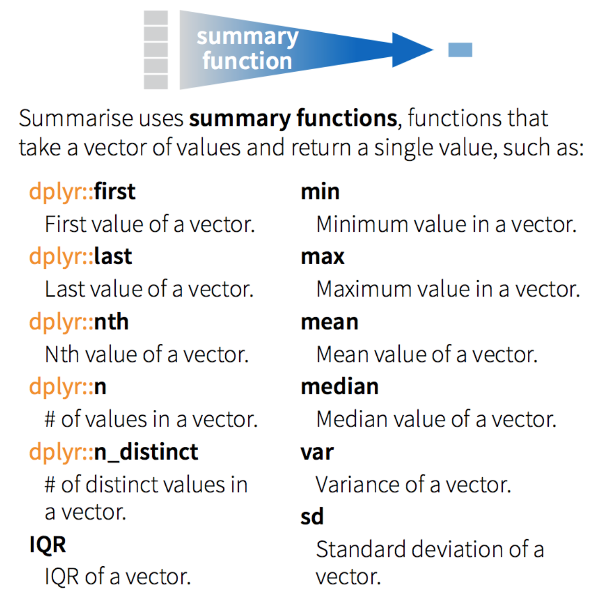
group_by() : group data frame by a factor for downstream operations (usually summarise)
summarise() : summarise values in a data frame or in groups within the data frame with aggregation functions (e.g. min(), max(), mean(), etc…)
dplyr - Split-Apply-Combine
The group_by function is key to the Split-Apply-Combine strategy
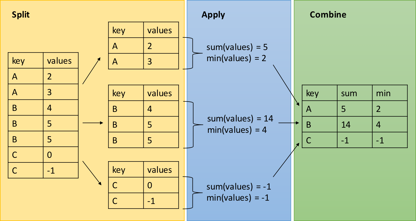
dplyr - Split-Apply-Combine
dplyr - Split-Apply-Combine
Example: we are interested in the mean temperature and standard deviation within each month if the airquality dataset
month_sum <- airquality %>% group_by(Month) %>% summarise(mean_temp = mean(Temp), sd_temp = sd(Temp))month_sum# # A tibble: 5 × 3# Month mean_temp sd_temp# <int> <dbl> <dbl># 1 5 65.5 6.85# 2 6 79.1 6.60# 3 7 83.9 4.32# 4 8 84.0 6.59# 5 9 76.9 8.36Challenge - dplyr and magrittr
Using the ChickWeight dataset, create a summary table which displays the difference in weight between the maximum and minimum weight of each chick in the study.
Employ dplyr verbs and the %>% operator.
## ?ChickWeightdata(ChickWeight)Solution
- Use
group_by()to divide the dataset byChick - Use
summarise()to calculate the weight gain within each group
weight_diff <- ChickWeight %>% group_by(Chick) %>% summarise(weight_diff = max(weight) - min(weight))head(weight_diff)# # A tibble: 6 × 2# Chick weight_diff# <ord> <dbl># 1 18 4# 2 16 16# 3 15 27# 4 13 55# 5 9 58# 6 20 76Ninja challenge
Using the
ChickWeightdataset, create a summary table which displays, for each diet, the average individual difference in weight between the end and the beginning of the study.Employ
dplyrverbs and the%>%operator.
Hint: first() and last() may be useful here
Ninja hint
Note that we can group the data frame using more than one factor, using
the general syntax as follows: group_by(group1, group2, ...)
Within group_by(), the multiple groups create a layered onion, and
each subsequent single use of the summarise() function peels off the
outer layer of the onion. In the above example, after we carried out a
summary operation on group2, the resulting data set would remain
grouped by group1 for downstream operations.
Ninja solution
diet_summ <- ChickWeight %>% group_by(Diet, Chick) %>% summarise(weight_gain = last(weight) - first(weight)) %>% group_by(Diet) %>% summarise(mean_gain = mean(weight_gain))diet_summ# # A tibble: 4 × 2# Diet mean_gain# <fct> <dbl># 1 1 115.# 2 2 174 # 3 3 230.# 4 4 188.R base challenge
Now try to redo the previous challenge only with functions from the R base!
Note that several solutions are possible.
Hint: the function ?aggregate() or ?by() may be useful here.
R base solution
weight_diff_rbase <- aggregate(weight ~ Chick, data = ChickWeight, FUN = function(x) weight_diff = max(x) - min(x))names(weight_diff_rbase) <- c("Chick", "weight_diff")# Is the r base output identical to the dplyr output?table(weight_diff_rbase == as.data.frame(weight_diff))# # TRUE # 100dplyr - Merging data frames
In addition to all the operations we have explored, dplyr also
provides some functions that allow you to join two data frames together.
The syntax in these functions is simple relative to alternatives in
other R packages:
left_join()right_join()inner_join()anti_join()
These are beyond the scope of the current introductory workshop, but they provide extremely useful functionality you may eventually require for some more advanced data manipulation needs.
Thank you for attending!
![]()
The argument
sep = "\\."tells R to splits the character string around the period (.). We cannot type directly"."because it is a regular expression that matches any single character.