Workshop 9: Multivariate analyses

# Workshop 9: Multivariate analyses
## QCBS R Workshop Series
### Québec Centre for Biodiversity Science

---

# About this workshop
[![badge](https://img.shields.io/static/v1?style=for-the-badge&label=repo&message=dev&color=6f42c1&logo=github)](https://github.com/QCBSRworkshops/workshop09)
[![badge](https://img.shields.io/static/v1?style=for-the-badge&label=wiki&message=09&logo=wikipedia)](https://wiki.qcbs.ca/r_workshop9)
[![badge](https://img.shields.io/static/v1?style=for-the-badge&label=Slides&message=09&color=red&logo=html5)](https://qcbsrworkshops.github.io/workshop09/workshop09-en/workshop09-en.html)
[![badge](https://img.shields.io/static/v1?style=for-the-badge&label=Slides&message=09&color=red&logo=adobe-acrobat-reader)](https://qcbsrworkshops.github.io/workshop09/workshop09-en/workshop09-en.pdf)
[![badge](https://img.shields.io/static/v1?style=for-the-badge&label=script&message=09&color=2a50b8&logo=r)](https://qcbsrworkshops.github.io/workshop09/workshop09-en/workshop09-en.R)

---

# Required packages

* [ape](https://cran.r-project.org/package=ape)
* [gclus](https://cran.r-project.org/package=gclus)
* [vegan](https://cran.r-project.org/package=vegan)

```R
install.packages(c('ape', 'gclus', 'vegan'))
```

---
# Learning objectives

##### Use R to perform an unconstrained ordination

#### Use R to create dendrogram

---

# 1. Introduction
## What is ordination?

---
# One Dimension

What if we are interested in this response for different species of algae involved in the algal bloom density?

---
# Two Dimensions

---
# Three Dimensions

---
# 4,5,6, or more Dimensions

---
# Ordination in reduced space

---
# Ordination in reduced space

- Matrix algebra is complex and hard to understand

- A global understanding is enough in order to use ordination methods adequately

---
# Methods for scientific research

--
- **Questions / Hypothesis**
--

- **Experimental design**

--
- **Data Collection**
--

- **Transformation / Distance**
--

- **Analysis**
--

- **Redaction**
--

- **Communication**

---
class: inverse, center, middle
# 2. Exploring data

---
# Doubs River Fish Dataset

Verneaux (1973) dataset:
- characterization of fish communities
- 27 different species
- 30 different sites
- 11 environmental variables

]

.pull.right[
![:scale 50%](images/DoubsRiver.png)
]

---
# Doubs River Fish Dataset

Load the Doubs River species data (Doubs.Spe.csv)

```r
spe <- read.csv("data/doubsspe.csv", row.names = 1)
spe <- spe[-8,] # remove site with no data
```

Load the Doubs River environmental data (Doubs.Env.csv)

```r
env <- read.csv("data/doubsenv.csv", row.names = 1)
env <- env[-8,] # remove site with no data
```

---
# Expore Doubs Dataset

Explore the content of the fish community dataset

```r
names(spe) # Names of objects
dim(spe) # dimensions
str(spe) # structure of objects
summary(spe) # summary statistics
head(spe) # first 6 rows
```

```
#   CHA TRU VAI LOC OMB BLA HOT TOX VAN CHE BAR SPI GOU BRO PER BOU PSO ROT CAR
# 1   0   3   0   0   0   0   0   0   0   0   0   0   0   0   0   0   0   0   0
# 2   0   5   4   3   0   0   0   0   0   0   0   0   0   0   0   0   0   0   0
# 3   0   5   5   5   0   0   0   0   0   0   0   0   0   1   0   0   0   0   0
# 4   0   4   5   5   0   0   0   0   0   1   0   0   1   2   2   0   0   0   0
# 5   0   2   3   2   0   0   0   0   5   2   0   0   2   4   4   0   0   2   0
# 6   0   3   4   5   0   0   0   0   1   2   0   0   1   1   1   0   0   0   0
#   TAN BCO PCH GRE GAR BBO ABL ANG
# 1   0   0   0   0   0   0   0   0
# 2   0   0   0   0   0   0   0   0
# 3   0   0   0   0   0   0   0   0
# 4   1   0   0   0   0   0   0   0
# 5   3   0   0   0   5   0   0   0
# 6   2   0   0   0   1   0   0   0
```

---
# Species Frequencies

Take a look at the distribution of species frequencies

```r
ab <- table(unlist(spe))
barplot(ab, las = 1, col = grey(5:0/5),
 xlab = "Abundance class", ylab = "Frequency")
```

---
# Species Frequencies

How many zeros?

```r
sum(spe == 0)
# [1] 408
```

What proportion of zeros?

```r
sum(spe == 0)/(nrow(spe)*ncol(spe))
# [1] 0.5210728
```

---
# Total Species Richness

Visualize how many species are present at each site:

```r
site.pre <- rowSums(spe > 0)
barplot(site.pre, main = "Species richness",
 xlab = "Sites", ylab = "Number of species",
 col = "grey ", las = 1)
```

---
# Understand your data!

- Are there many zeros?

- What do they mean?

---
# Before transforming your community data...

--
- relative abundances/counts/presence-absence?

--
- asymmetrical distributions?

--
- many rare species?

--
- overabundance of dominant species?

--
- double Zero problem?

---
# Transforming community data

---
# Transforming your community data

## Examples

Transforming counts into presence - absence

```r
library(vegan)
spec.pa <- decostand(spe, method = "pa")
```

Reducing the weight of rare species

```r
spec.hel <- decostand(spe, method = "hellinger")
spec.chi <- decostand(spe, method = "chi.square")
```

Reducing the weight of very abundant species

```r
spe.pa <- decostand(spe,method = "log")
```

---
# Doubs Environmental Data

```r
names(env) # Names of objects
dim(env) # dimensions
str(env) # structure of objects
summary(env) # summary statistics
head(env) # first 6 rows
```

```r
head(env) # first 6 rows
#    das alt  pen  deb  pH dur  pho  nit  amm  oxy dbo
# 1  0.3 934 48.0 0.84 7.9  45 0.01 0.20 0.00 12.2 2.7
# 2  2.2 932  3.0 1.00 8.0  40 0.02 0.20 0.10 10.3 1.9
# 3 10.2 914  3.7 1.80 8.3  52 0.05 0.22 0.05 10.5 3.5
# 4 18.5 854  3.2 2.53 8.0  72 0.10 0.21 0.00 11.0 1.3
# 5 21.5 849  2.3 2.64 8.1  84 0.38 0.52 0.20  8.0 6.2
# 6 32.4 846  3.2 2.86 7.9  60 0.20 0.15 0.00 10.2 5.3
```

Explore colinearity by visualizing correlations between variables

```r
pairs(env, main = "Bivariate Plots of the Environmental Data")
```

---
# Doubs Environmental Data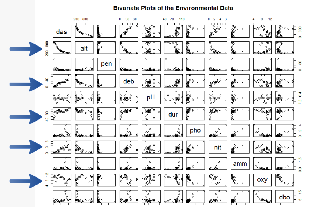

![](images/EnvDat1.png)

---
# Standardization

Standardizing environmental variables is crucial as you cannot compare the effects of variables with different units

```r
## ?decostand
env.z <- decostand(env, method = "standardize")
```

This centers and scales the variables to make your downstream analysis more appropriate

```r
apply(env.z, 2, mean)
#           das           alt           pen           deb            pH 
# -7.959539e-17 -4.795165e-17  2.494600e-17 -7.323225e-17 -1.730430e-15 
#           dur           pho           nit           amm           oxy 
# -2.028505e-16  4.445790e-17  2.875893e-17  2.754434e-17 -4.038167e-16 
#           dbo 
#  9.829975e-17
apply(env.z, 2, sd)
# das alt pen deb  pH dur pho nit amm oxy dbo 
#   1   1   1   1   1   1   1   1   1   1   1
```

---
class: inverse, center, middle
# 3. Similarity / Dissimilarity

---
# Association measures

Matrix algebra is at the heart of all ordinations

- Exploring various measures of distance between objects provides some understanding of the engine under the hood

---
# Breaking out of 1D

- As you have seen, ecological datasets can sometimes be very large matrices

- Ordinations compute the relationships between species or between sites

- We can simplify these relationships using methods of dissimilarity
]

![:scale 40%](images/PCAMatrix.png)

![:scale 40%](images/distMes.png)

![:scale 40%](images/distMat.png)
]

---
# Similarity / Dissimilarity

- Useful to understand your dataset
- Appropriate measure required by some types of ordinations

![](images/similarity.png)

---
# Community distance measures

--

---
# Comparing Doubs Sites

The `vegdist()` function contains all common distances

```r
?vegdist
```

How different is the community composition across the 30 sites of the Doubs River?

```r
spe.db.pa <- vegdist(spe, method = "bray")
```

---
# Comparing Doubs Sites

---
# Comparing Doubs Sites

---
# Visualization of distance matrices

---
# Challenge #1 ![:cube]()

Discuss with your neighbor:

- Make a list of all your suggestions

---
# And what about ordination?

With ordination methods, we order our objects (site) according to their similarity

- The more the sites are similar, the closer they are in the ordination space (smaller distances)

- In Ecology, we usually calculate the similarity between sites according to their species composition or their environmental conditions.

---
# Schematic analysis of multivariate analysis

---
# Clustering

- To highlight structures in the data by partitioning either objects or the descriptors

- Results are represented as dendrograms (trees)

- Not a statistical method

---
# Overview of 3 hierarchical methods

- Single linkage agglomerative clustering

- Complete linkage, agglomerative clustering

- Ward's minimum variance clustering

- Elements of lower are nested in higher ranking clusters
   - (e.g. species, genus, family, order)

---
# Hierarchical methods

A distance matrix is first sorted in increasing distance order

![](images/Hierachic1.png)

---
# Single linkage clustering

![:scale 50%](images/singleClust1.png)
--

]

- The two closest objects merge

- The next two closest objects/clusters merge

- and so on

![](images/singleClust2.png)

]

---
# Complete linkage clustering

![:scale 50%](images/compleClust1.png)

]

- The two closest objects merge

- The next two objects/cluster will agglomerate when linked to the furthest element of the group

![](images/compleClust2.png)
]

---
# Comparison

Create a distance matrix from Hellinger transformed Doubs river data and compute the single linkage clustering

```r
spe.dhe1 <- vegdist(spec.hel, method = "euclidean")
spe.dhe1.single <- hclust(spe.dhe1, method = "single")
plot(spe.dhe1.single)
```

---
# Comparison

![](images/comparison.png)

**Single linkage:**

Chains of objects occur (e.g. 19,29,30,26)
]

**Complete linkage:**
Contrasted groups are formed of objects occur
]

---
# Ward's minimum variance method

- Uses the criterion of least squares to cluster objects into groups
  - At each step, the pair of clusters merging is the one leading to the minimum increase in total within-group sum of squares

---
# Ward's method

Compute the Ward's minimum variance clustering and plot the dendrogram by using the square root of the distances:

```r
spe.dhel.ward <- hclust(spe.dhe1, method = "ward.D2")
spe.dhel.ward$height <- sqrt(spe.dhel.ward$height)
plot(spe.dhel.ward, hang = -1) # hang = -1 aligns objects at the same level
```

---
# Ward's method

Clusters generated using this method tend to be more spherical and to contain similar number of objects

---
# How to choose the right method?

- Depends on the objective
  - highlights gradients? contrasts?
- If more than on method seems appropriate, compare dendrograms
- Again: this is **not** an statistical method
 But! is possible to:
  - determine the optimal number of interpretable clusters
  - compute clustering statistics
  - combine clustering to ordination to distinguish groups of sites

---
class: inverse, center, middle
# 4. Unconstrained ordination

---
# Definitions

- **Variance:** measure of a variable `$y_j$` dispersion from its mean
--

- **Co-variance:** measure of co-dispersion of variables `$y_j$` et `$y_i$` from their means

--
- **Correlation:** measure of the link strength between 2 variables: `$r_{ij} = (d_{ij} / d_j x d_k)$`

--
- **Eigenvalues:** Proportio of variance (dispersion) represented by one ordination axe.

--
- **Orthogonality:** right angle between 2 axis or 2 arrows which means that these 2 are independent = non correlated.

--
- **Score:** position of a dot on an axis. All the scores of a dot give its coordinates in the multidimensional space. They can be used as new variable for other analyses (e.g. linear combination of measured variables).

--
- **Dispersion** (inertia): Measure of the total variability of the scatter plot (descriptors) in the multidimensional space with regards to its center of gravity.

---
# Unconstrained ordination

- Asses relationships **within** a set of variables (species or environmental variables, not **between** sets, i.e. constrained analysis)

- Find key components of variation between samples, sites, species, etc... ç

- Reduce the number of dimensions in multivariate data without substantial loss of information

- Create new variables for use in subsequent analysis (such as regression)

---
# 4.1. Principal Component Analysis (PCA)

- Preserves, in 2D, the maximum amount of variation in the data
- The resulting, synthetic variables are orthogonal (and therefore uncorrelated)

---
# PCA - What you need

- A set of variables that are response variables (e.g. community composition) OR explanatory variables (e.g. environmental variables)

**NOT BOTH!**

.pull-left[
- Samples that are measured for the same set of variables
- Generally a dataset that is longer than it is wide is preferred
]

---
# PCA - Walkthrough

|Site|Species 1| Species 2|
|---|------|------|
|A|7|3|
|B|4|3|
|C|12|10|
|D|23|11|
|E|13|13|
|F|15|16|
|G|18|14|

---
# PCA - Walkthrough

.small[
.alert[In 2D, we would plot the sites like this... Notice the dispersion in the scatterplot]]

---
# PCA - Walkthrough

.small[
.alert[Our first component is essentially drawn trough the maximum amount of observed variation... or the best fit line through the points]]

---
# PCA - Walkthrough

.center[
![:scale 70%](images/PCA2.png)]
.small[
.alert[A second principal component is then added perpendicular (90 degrees in 2D) to the first axis]]

---
# PCA - Walkthrough

.small[ The final plot then is the two PC axes rotated where the axes are now principal components as opposed to species]
---
# PCA - Multidimensional case

- **PC1** --> axis that maximizes the variance of the points that are projected perpendicularly onto the axis.
- **PC2** --> must be perpendicular to PC1, but the direction is again the one in which variance is maximized when points are perpendicularly projected
- **PC3** --> and so on: perpendicular to the first two axes

.alert[When there are more than two dimensions, PCA produces a new spaces in which all PCA axes are orthogonal (i.e. non-correlated)  and where the PCA axes are ordered according to the percent of variance of the original data they explain]

---
# PCA - Let's try it on Fish Species!

- For both PCA and RDA, we will be using the `rda()` function in the vegan package

- Run a PCA on the Hellinger-transformed fish data and extract the results

```r
spe.h.pca <- rda(spec.hel)

summary(spe.h.pca)
# 
# Call:
# rda(X = spec.hel) 
# 
# Partitioning of variance:
#               Inertia Proportion
# Total          0.5025          1
# Unconstrained  0.5025          1
# 
# Eigenvalues, and their contribution to the variance 
# 
# Importance of components:
#                          PC1     PC2     PC3     PC4     PC5     PC6     PC7
# Eigenvalue            0.2580 0.06424 0.04632 0.03850 0.02197 0.01675 0.01472
# Proportion Explained  0.5133 0.12784 0.09218 0.07662 0.04371 0.03334 0.02930
# Cumulative Proportion 0.5133 0.64118 0.73337 0.80999 0.85370 0.88704 0.91634
#                           PC8      PC9     PC10     PC11     PC12     PC13
# Eigenvalue            0.01156 0.006936 0.006019 0.004412 0.002982 0.002713
# Proportion Explained  0.02300 0.013803 0.011978 0.008781 0.005935 0.005399
# Cumulative Proportion 0.93934 0.953144 0.965123 0.973903 0.979838 0.985237
#                           PC14     PC15     PC16      PC17      PC18      PC19
# Eigenvalue            0.001835 0.001455 0.001118 0.0008309 0.0005415 0.0004755
# Proportion Explained  0.003651 0.002895 0.002225 0.0016535 0.0010776 0.0009463
# Cumulative Proportion 0.988888 0.991783 0.994008 0.9956612 0.9967389 0.9976852
#                            PC20      PC21      PC22      PC23      PC24
# Eigenvalue            0.0003680 0.0002765 0.0002253 0.0001429 7.618e-05
# Proportion Explained  0.0007324 0.0005503 0.0004483 0.0002845 1.516e-04
# Cumulative Proportion 0.9984176 0.9989678 0.9994161 0.9997006 9.999e-01
#                           PC25      PC26      PC27
# Eigenvalue            4.99e-05 1.526e-05 9.118e-06
# Proportion Explained  9.93e-05 3.036e-05 1.814e-05
# Cumulative Proportion 1.00e+00 1.000e+00 1.000e+00
# 
# Scaling 2 for species and site scores
# * Species are scaled proportional to eigenvalues
# * Sites are unscaled: weighted dispersion equal on all dimensions
# * General scaling constant of scores:  1.93676 
# 
# 
# Species scores
# 
#          PC1      PC2       PC3        PC4        PC5       PC6
# CHA  0.17336  0.08295 -0.064963  0.2539861 -0.0285801  0.019057
# TRU  0.64860  0.01162 -0.261994 -0.1606020 -0.0745819 -0.088616
# VAI  0.51810  0.14773  0.165304  0.0241017  0.1012928  0.104748
# LOC  0.38606  0.16615  0.242995 -0.0275216  0.1258011  0.048299
# OMB  0.16893  0.06274 -0.096143  0.2426514  0.0140574  0.062117
# BLA  0.07786  0.14644 -0.031402  0.2339394 -0.1032338 -0.040810
# HOT -0.18491  0.04901 -0.045107  0.0199377  0.0687305  0.009650
# TOX -0.14644  0.17834 -0.010937  0.0649955 -0.0006229 -0.106955
# VAN -0.11436  0.15673  0.142223 -0.0127266 -0.1989404  0.013897
# CHE -0.09682 -0.15449  0.242943  0.1124210  0.0233830 -0.039996
# BAR -0.19826  0.21211 -0.053980  0.0969899  0.0067098 -0.035442
# SPI -0.17689  0.16250 -0.033112  0.0397113  0.0323159 -0.072908
# GOU -0.23138  0.09782  0.064144 -0.0013887 -0.1503303  0.130575
# BRO -0.15129  0.12804  0.040303 -0.1203826 -0.1006077  0.066242
# PER -0.15719  0.18144  0.057029 -0.0940032 -0.0412984 -0.060409
# BOU -0.22853  0.13870 -0.062197 -0.0125024  0.0798647 -0.006907
# PSO -0.22790  0.08231 -0.065797  0.0172143  0.0611434 -0.001407
# ROT -0.19221  0.03090 -0.006264 -0.0739133 -0.0731548  0.074581
# CAR -0.18699  0.13388 -0.050804  0.0001803  0.0403961 -0.031005
# TAN -0.19169  0.15719  0.114415 -0.0818330  0.0142624 -0.072024
# BCO -0.20174  0.08807 -0.067086 -0.0529106  0.0737228  0.037312
# PCH -0.14717  0.05829 -0.067311 -0.0458414  0.0501013  0.031605
# GRE -0.30155 -0.01785 -0.084333 -0.0181797  0.0226500  0.126639
# GAR -0.35245 -0.14076  0.168014  0.0185946  0.0213462 -0.129788
# BBO -0.24317  0.03679 -0.082731 -0.0384489  0.0939828  0.063369
# ABL -0.42536 -0.26155 -0.054190  0.1021959 -0.0078085  0.044540
# ANG -0.20631  0.11889 -0.062079 -0.0175733  0.0718743 -0.001956
# 
# 
# Site scores (weighted sums of species scores)
# 
#          PC1      PC2      PC3      PC4       PC5       PC6
# 1   0.367401 -0.39935 -1.08857 -0.63304 -0.512027 -0.858378
# 2   0.503582 -0.05683 -0.19259 -0.43441  0.389533  0.069451
# 3   0.461709  0.02262 -0.06522 -0.49798  0.309425  0.270577
# 4   0.298336  0.15130  0.26748 -0.53196  0.003088  0.184821
# 5  -0.002222  0.07631  0.54769 -0.50936 -0.780261 -0.169353
# 6   0.212816  0.08345  0.55091 -0.42210 -0.139518 -0.104278
# 7   0.438055 -0.06114  0.15590 -0.31150  0.158686  0.036565
# 9   0.040794 -0.44269  0.89022  0.09609  0.641193 -0.646943
# 10  0.298011 -0.01094  0.56837 -0.10013 -0.088124  0.515072
# 11  0.467609 -0.12622 -0.15505  0.29459  0.325464  0.200912
# 12  0.476845 -0.07691 -0.16329  0.29384  0.360112  0.194576
# 13  0.483620  0.06649 -0.44723  0.53734  0.048587  0.182565
# 14  0.371728  0.16555 -0.21939  0.62130 -0.183604  0.364847
# 15  0.277048  0.23525  0.08928  0.61773 -0.475769  0.124107
# 16  0.077024  0.47455  0.17116  0.34361 -0.570434 -0.572740
# 17 -0.053860  0.42290  0.02810  0.42376 -0.059203 -0.586419
# 18 -0.135418  0.37780  0.03233  0.39706 -0.007199 -0.347064
# 19 -0.269281  0.30751  0.18022  0.09354  0.178657 -0.016299
# 20 -0.378830  0.19764  0.04939 -0.03438  0.157660 -0.056696
# 21 -0.409369  0.22888 -0.08401 -0.12823  0.152787  0.096105
# 22 -0.443679  0.17698 -0.13708 -0.13152  0.103294  0.030004
# 23 -0.242292 -1.11711  0.15254  0.40512  0.045573 -0.576778
# 24 -0.358333 -0.83372 -0.17314  0.27200  0.181192  0.347231
# 25 -0.325288 -0.61983  0.10487  0.01059 -1.034438  0.750325
# 26 -0.441703  0.02111 -0.13742 -0.14346  0.200775  0.244356
# 27 -0.444529  0.12735 -0.15915 -0.14112  0.179240  0.123487
# 28 -0.446407  0.12774 -0.18830 -0.15467  0.239617  0.117101
# 29 -0.355788  0.28044 -0.28006 -0.02003  0.110181  0.079568
# 30 -0.467578  0.20086 -0.29797 -0.21269  0.065512  0.003276
```

---
# Function `rda()`

- RDA is in 2 steps

- multiple regressions
  - PCA on regressed values

- If we give only one table to the function `rda()` it does directly a PCA without doing regression

rda(Y) or rda(X) ![:faic](arrow-right) PCA ]]

---
#PCA - Interpretation of Output

- Total variance explained by the descriptors (here the fish species)
- In PCA, not that the "Total" and "Unconstrained" portion of the explained variance is identical