About this workshop


What is R?
Ris a free an open-source programming language and environment.
- It is designed for data analysis, graphical display and data simulations.
- It is one of the world's leading statistical programming environments.
![]()
Why should I become an useR?
Ris free, open source: built for you and for everyone;Ris popular: a large enganged user-base fosters the continued development and the maintainance of statistical tools;Ris powerful- You can program complex simulations
- Use it on high performance clusters
Rsupports extensionsRruns on most operating systemsRconnects with other languages:C++,Java,Python,Julia,Stanand more!

Why use R?
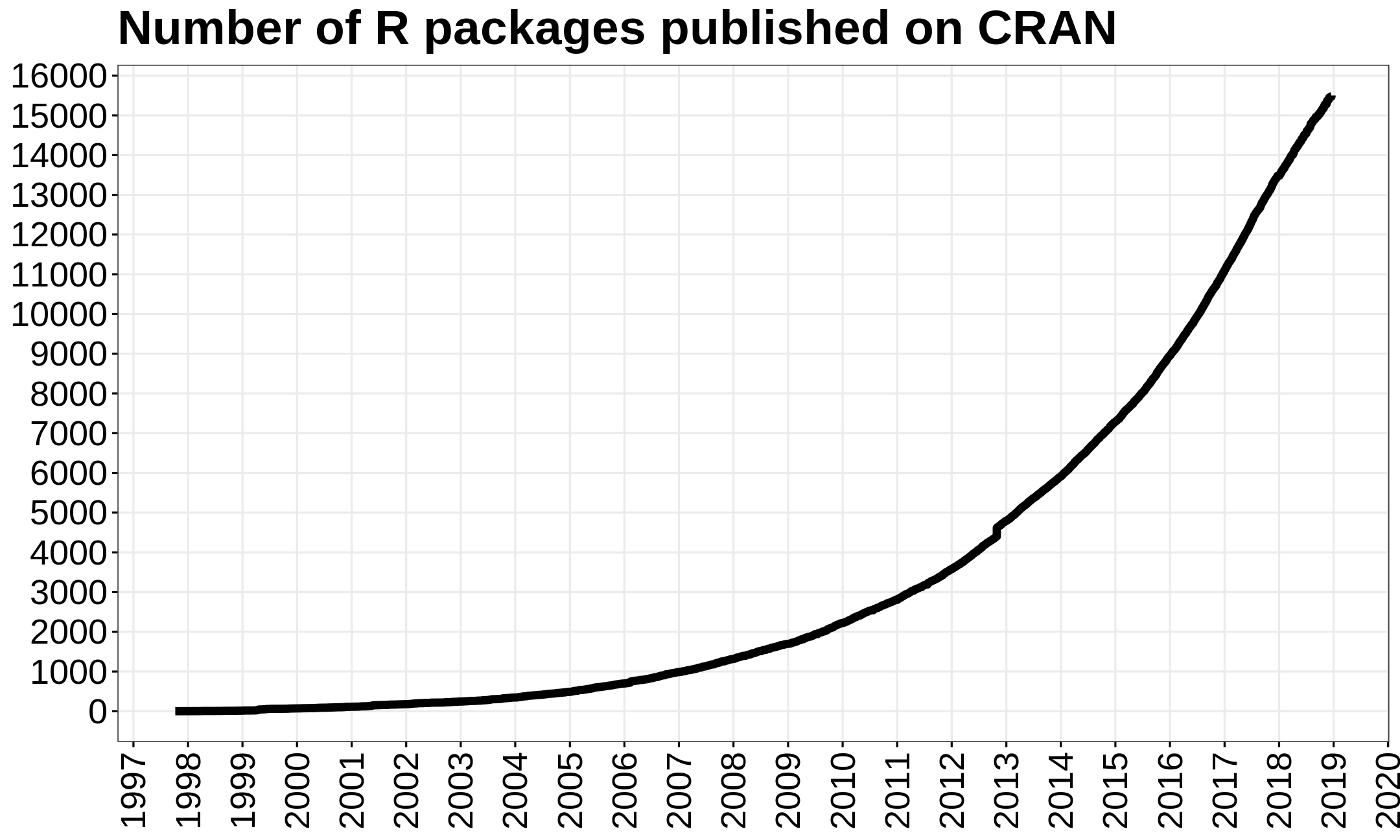
- More and more scientists use it every year!
- As of October 2020, there are more than 16000 packages registered within the Comprehensive R Archive Network (CRAN) (and thousands more within Github repositories)!
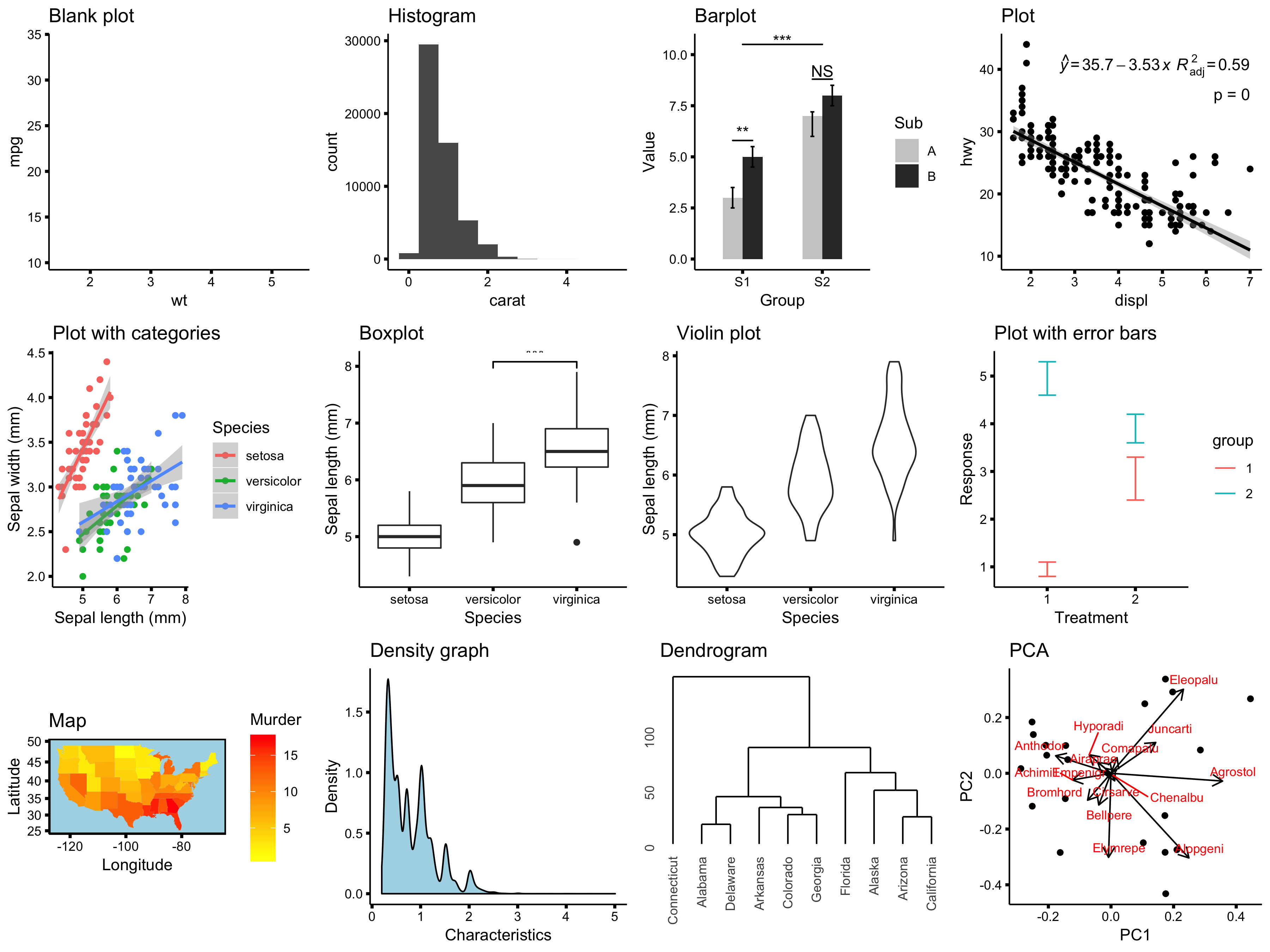
A lot of features: customizable graphs
All of these graphs were made in R!
And what about RStudio?
RStudio is the most used Integrated Development Environment (IDE) for R.
It includes a console, a syntax-highlighting editor that supports direct code execution with tools for plotting, history, debugging and workspace management.
It integrates with R (and other programming languages) to provide a lot of useful features:
RStudio supports authoring HTML, PDF, Word and presentation documents
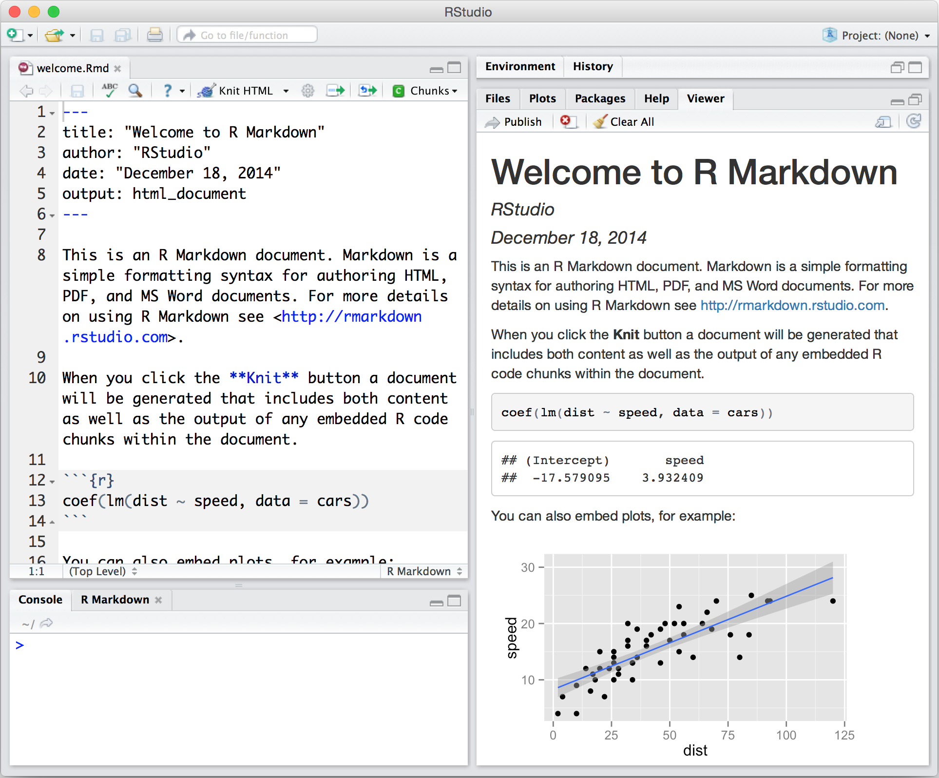
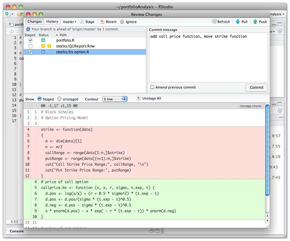
RStudio supports version control with Git (directly to Github) and Subversion
And what about RStudio?
RStudio is the most used Integrated Development Environment (IDE) for R.
It includes a console, a syntax-highlighting editor that supports direct code execution with tools for plotting, history, debugging and workspace management.
It integrates with R (and other programming languages) to provide a lot of useful features:
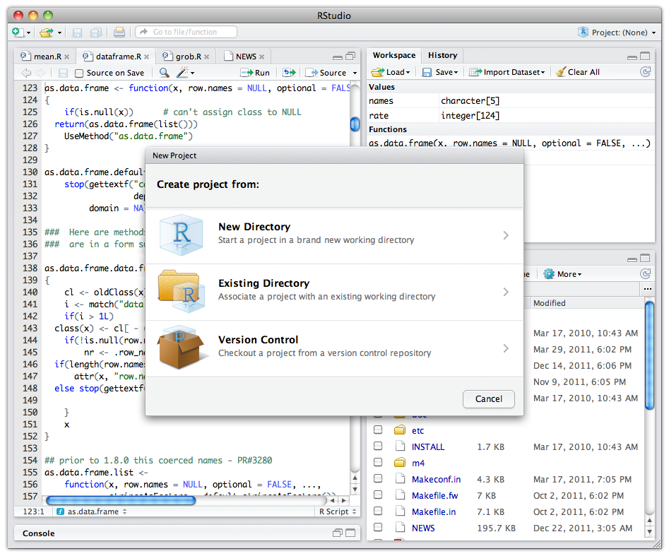
RStudio make it easy to start new or find existing projects
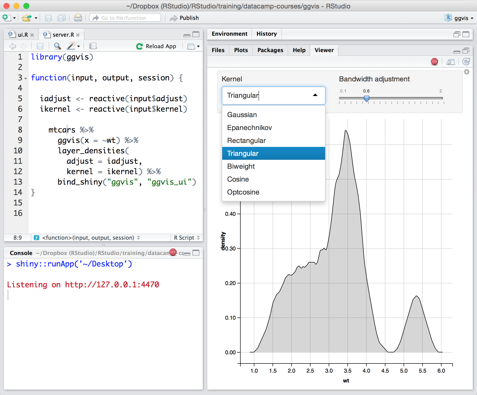
RStudio supports interactive graphics with Shiny and ggvis
And what about RStudio?
RStudio is the most used Integrated Development Environment (IDE) for R.
It includes a console, a syntax-highlighting editor that supports direct code execution with tools for plotting, history, debugging and workspace management.
It integrates with R (and other programming languages) to provide a lot of useful features:
RStudio make it easy to start new or find existing projects
RStudio supports interactive graphics with Shiny and ggvis
There are other IDE for R: Atom, Visual Studio, Jupyter notebook and Jupyter lab!
Challenge
- Throughout these workshops, challenges will be indicated by Rubik cubes.
- Sometimes, you will be expected to collaborate with other participants!
- Do not hesitate to ask questions!
First Challenge
Open RStudio.
Let us do this one together!

The RStudio Interface
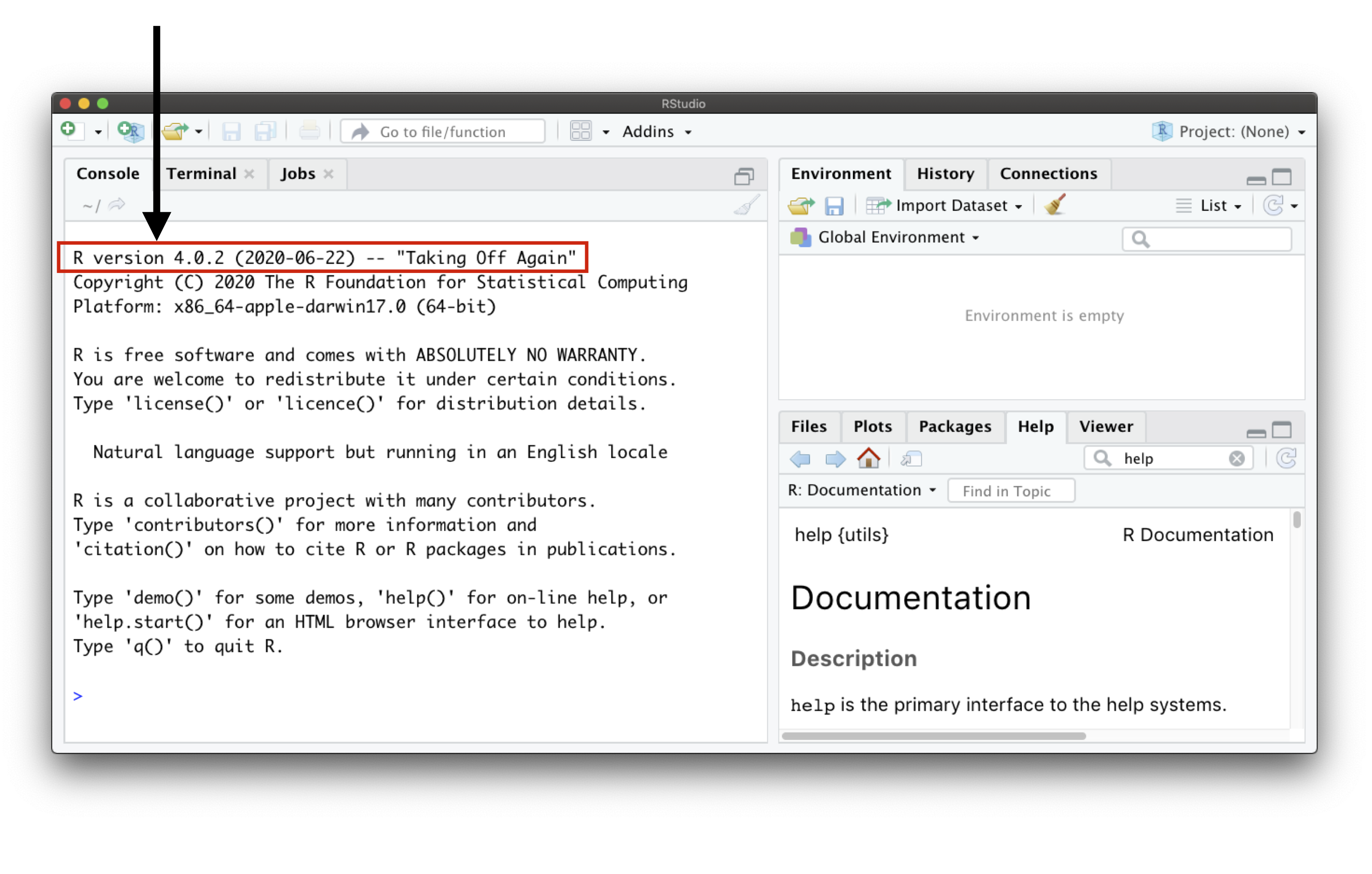
When you open RStudio for the first time, the screen will be divided across three main Pane groups:
- Console, Terminal, Job group;
- Environment, History, Connections group;
- Files, Plot, Packages, Help, Viewer panes; and,
- Script pane group.
Once you Open a Script or Create a New Script (File > New File > R Script or Ctrl/Cmd + Shit + N), the fourth panel will appear!

The RStudio Console
Usually, the first text you see within the Console pane is the
Rversion RStudio is using.The Console is the place where
Ris waiting for you to tell it what to do, and is where it will communicate with you, showing the outcome of your command.Whenever
Ris ready to accept commands, it will show a>prompt.
Challenge
Use R to calculate the following equation:
2+16∗24−56
Hint: The * symbol is used to multiply.
Challenge: Solution
Use R to calculate the following equation:
2+16∗24−56
It would look like this in R:
2 + 16 * 24 - 56# [1] 330Challenge
Use R to calculate the following equation:
2+16∗24−56/(2+1)−457
Hint: Think about the order of the operation.
Challenge: Solution
Use R to calculate the following equation:
2+16∗24−56/(2+1)−457
It would look like this in R:
2 + 16 * 24 - 56 / (2 + 1) - 457# [1] -89.66667Note that R respects the order of the operations
Still using R for arithmetic operations
What is the area of a circle with a radius of 5 cm?
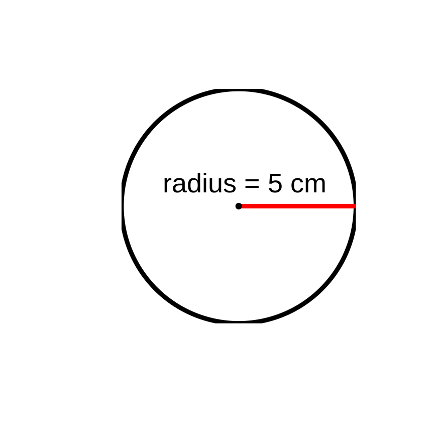
Areacircle=π×r2
Still using R for arithmetic operations
What is the area of a circle with a radius of 5 cm?

Areacircle=π×r2
3.1416 * 5^2# [1] 78.54Still using R for arithmetic operations
What is the area of a circle with a radius of 5 cm?
Areacircle=π×r2
3.1416 * 5^2# [1] 78.54But... R has built-in constants!
You can find them by typing ? and Constants (as in ?Constants) and executing it! What is the one for π?
We can then write and execute this:
pi * 5^2# [1] 78.53982You have just ran a command preceeded by ?. What happened?
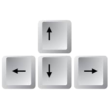
A tip
We can use the ↑ and ↓ arrow keys to retrieve commands previously run.
Make sure your cursor is blinking in front of the > prompt and give it a try!
Challenge
Create an object with a name (of your choice) that starts with a number. What happens?
Challenge: Solution
Create an object with a name (of your choice) that starts with a number. What happens?
Creating an object name that starts with a number returns the following error:
Error: unexpected symbol in "your object name"Challenge
Create an object with a value of 1 + 1.718282 (e or Euler's number) and name it euler_value.
Challenge: Solution
Create an object with a value of 1 + 1.718282 (e or Euler's number) and name it euler_value.
euler_value <- 1 + 1.718282euler_value# [1] 2.718282Challenge: Solution
Create an object with a value of 1 + 1.718282 (e or Euler's number) and name it euler_value.
euler_value <- 1 + 1.718282euler_value# [1] 2.718282What has happened in your RStudio window when you created this object?
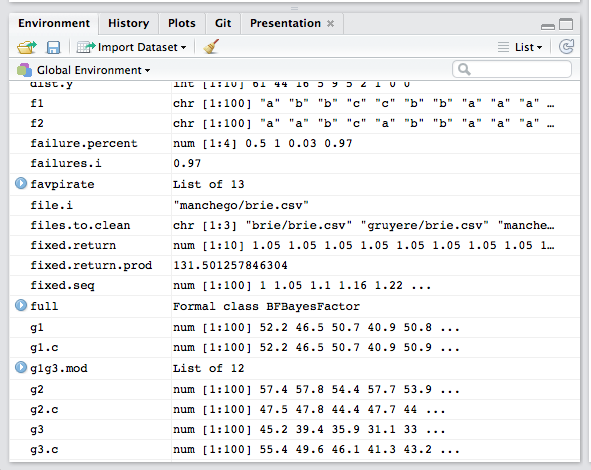
The RStudio Environment
The Environment panel shows you all the objects you have defined in your current workspace.
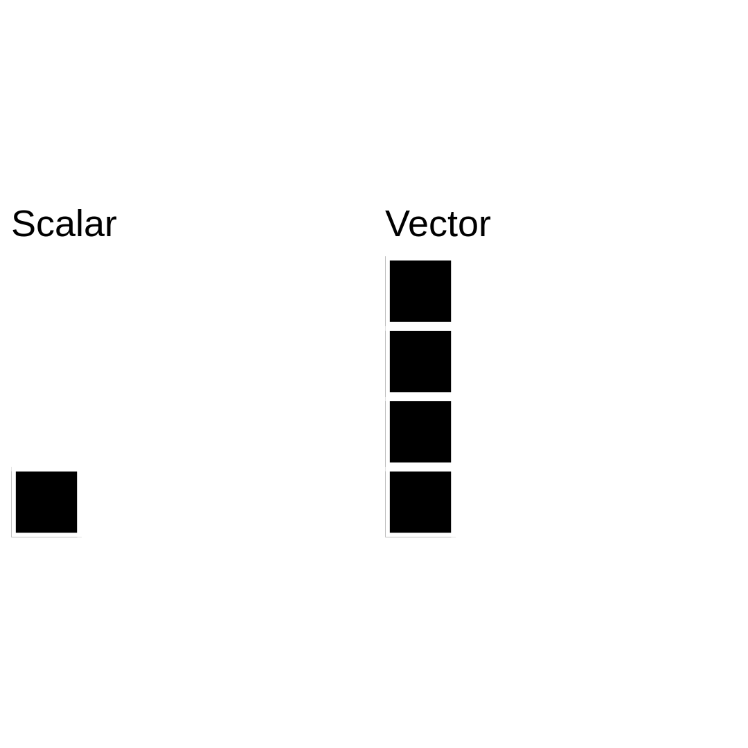
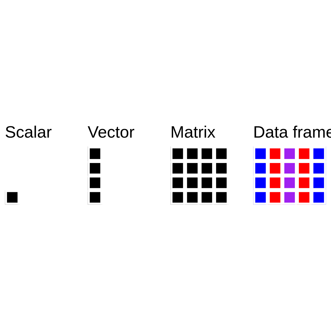
Data structure in R: vectors
A vector object is just a combination of several scalars stored as a single object.
Like scalars, vectors can be of numeric-, logical-, character-types, but never a mix of them!
Challenge
Let's practice:
- Create a vector containing the first 5 odd numbers, starting from 1
- Name it
odd_n - You can use any of the previous functions we have previously learned!
Challenge: Solution
Let's practice:
- Create a vector containing the first 5 odd numbers, starting from 1
- Name it
odd_n - You can use any of the previous functions we have previously learned!
Solution:
odd_n <- c(1, 3, 5, 7, 9)or
odd_n <- seq(from = 1, to = 9, by = 2)odd_n# [1] 1 3 5 7 9Data structure in R: matrices
We have learned that scalars contain one element, and that vectors contain more than one scalar of the same type!
Matrices are nothing but a bunch of vectors stacked together!
While vectors have one dimension, matrices have two dimensions, determined by rows and columns.
Finally, like vectors and scalars matrices can contain only one type of data: numeric, character, or logical.

Challenge
It is your time to get your hands dirty!
- Create an object containing a matrix with 2 rows and 3 columns, with values from 1 to 6, sorted per column.
- Create another object with a matrix with 2 rows and 3 columns, with the names of six animals you like.
- Create a third object with 4 rows and 2 columns:
- in the first column, include the numbers from 2 to 5; and,
- in the second column, include the first name of participants in this workshop.
- Compare them and tell us what differences have you detected (despite their values).
Remember that text strings must always be surrounded by quote marks (" ").
Remember that values or arguments must be separated by commas if they are inside a function, e.g. c("one", "two", "three").
Challenge
It is your time to get your hands dirty!
- Create an object containing a matrix with 2 rows and 3 columns, with values from 1 to 6, sorted per column.
- Create another object with a matrix with 2 rows and 3 columns, with the names of six animals you like.
(step_1 <- matrix(data = 1:6, nrow = 2, ncol = 3))# [,1] [,2] [,3]# [1,] 1 3 5# [2,] 2 4 6(step_2 <- matrix( data = c("cheetah", "tiger", "ladybug", "deer", "monkey", "crocodile"), nrow = 2, ncol = 3))# [,1] [,2] [,3] # [1,] "cheetah" "ladybug" "monkey" # [2,] "tiger" "deer" "crocodile"Challenge
It is your time to get your hands dirty!
- Create a third object with 4 rows and 2 columns:
- in the first column, include the numbers from 2 to 5; and,
- in the second column, include the first name of participants in this workshop.
- Compare them and tell us what differences have you detected (despite their values).
step_1# [,1] [,2] [,3]# [1,] 1 3 5# [2,] 2 4 6step_2# [,1] [,2] [,3] # [1,] "cheetah" "ladybug" "monkey" # [2,] "tiger" "deer" "crocodile"step_3 <- cbind(c(2:5), c("linley", "jessica", "joe", "emma"))step_3# [,1] [,2] # [1,] "2" "linley" # [2,] "3" "jessica"# [3,] "4" "joe" # [4,] "5" "emma"Data structure in R: data frames
Differently than a matrix, a data frame can contain numeric, character, and logical columns (or vectors).
Challenge
Using the vector num_vector and our indexing abilities:
- Extract the 4th value;
- Extract the 1st and 3rd values;
- Extract all values except for the 2nd and the 4th;
- Extract from the 6th to the 10th value.
num_vector <- c(1, 4, 3, 98, 32, -76, -4)Challenge: Solution
Using the vector num_vector and our indexing abilities:
- Extract the 4th value
num_vector[4]# [1] 98- Extract the 1st and 3rd values
num_vector[c(1, 3)]# [1] 1 3- Extract all values except for the 2nd and the 4th
num_vector[c(-2, -4)]# [1] 1 3 32 -76 -4- Extract from the 6th to the 10th value.
num_vector[6:10]# [1] -76 -4 NA NA NA
What happened there? What is that NA?
Indexing from matrices and data frames
To index a data frame you must specify the position of values within two dimensions: within the row and columns, as in:
data_frame_name[row_number, column_number]In this way, to extract the first row:
my_df[1, ]To extract the third column:
my_df[, 3]And, to extract the element within the second row and the fourth column:
my_df[2, 4]
Battleship (game) feelings!
Challenge
Explore the difference between these two lines of code:
char_vector == "blue"char_vector[char_vector == "blue"]Challenge: Solution
Explore the difference between these 2 lines of code:
char_vector == "blue"# [1] TRUE FALSE FALSEIn this line of code, you test a logical statement. For each entry in the char_vector, R checks whether the entry is equal to blue or not.
char_vector[char_vector == "blue"]# [1] "blue"In this above line, we asked R to extract all values within the char_vector vector that are exactly equal to blue.
Challenge
Extract the
num_spcolumn fromsoil_fertilisation_dataand multiply its value by the first four values ofnum_vec.After that, write a statement that checks if the values you obtained are greater than 25.
Challenge: Solution
- Extract the
num_spcolumn fromsoil_fertilisation_dataand multiply its value by the first four values ofnum_vec.
soil_fertilisation_data$num_sp * num_vector[c(1:4)]# [1] 17 92 45 686or
soil_fertilisation_data[, 3] * num_vector[c(1:4)]# [1] 17 92 45 686- After that, write a statement that checks if the values you obtained are greater than 25.
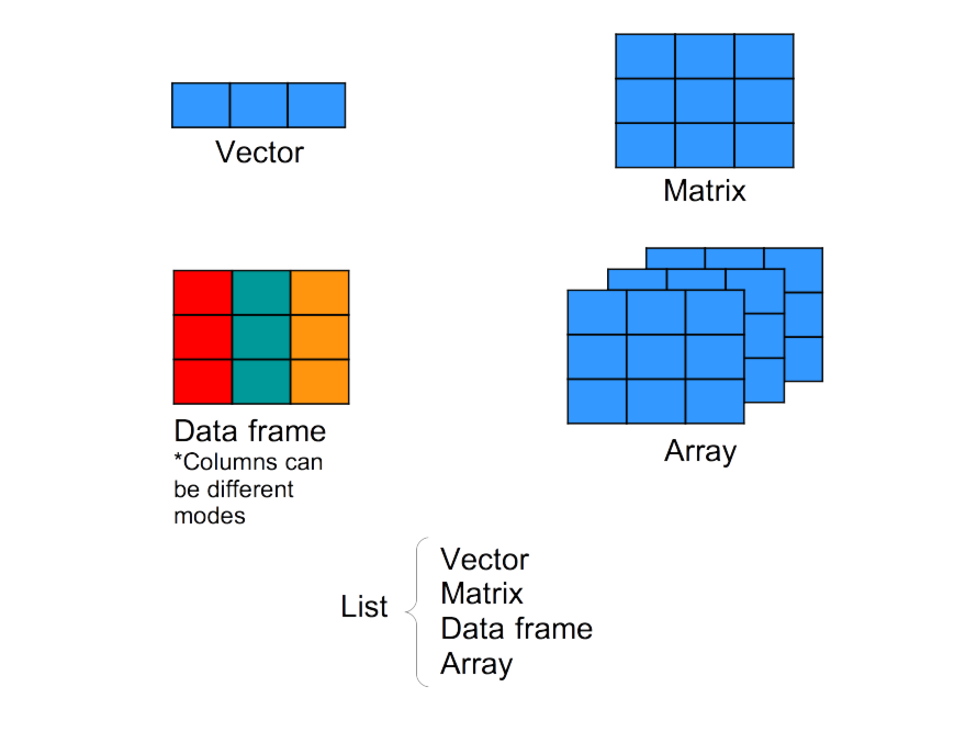
(soil_fertilisation_data$num_sp * num_vector[c(1:4)]) > 25# [1] FALSE TRUE TRUE TRUEOther kinds of data structure: arrays and lists
We focused here mainly on vectors and data frames.
While we will discuss discuss about arrays and lists in other workshops, you can already have an idea what these types of object structure are.
Any wild guesses?
Short review about data structure in R

Functions
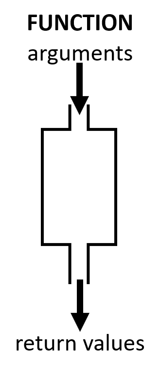
A function is a tool that simplifies our lives!
It allows you to quickly execute operations on objects without having to write every mathematical step.
A function needs entry values called arguments (or parameters).
It then performs (hidden) actions using these arguments and returns an output.
Today, we will look only into
R's built-in functions, but you will learn how to make your own functions during Workshop #5!
Challenge
- Create a vector
athat contains all the numbers from 1 to 5. - Create an object
bthat has a value of 2. - Add
aandbtogether using the basic+operator and save the result in an object calledresult_add. - Add
aandbtogether using thesumfunction and save the result in an object calledresult_sum. - Are
result_addandresult_sumdifferent? - Add
5toresult_sumusing thesum()function.
Challenge: Solution
- Are
result_addandresult_sumdifferent?
a <- c(1:5)b <- 2result_add <- a + bresult_sum <- sum(a, b)- Add
5toresult_sumusing thesum()function.
result_add# [1] 3 4 5 6 7result_sum# [1] 17sum(result_sum, 5)# [1] 22Challenge: Solution
- Are
result_addandresult_sumdifferent?
a <- c(1:5)b <- 2result_add <- a + bresult_sum <- sum(a, b)- Add
5toresult_sumusing thesum()function.
result_add# [1] 3 4 5 6 7result_sum# [1] 17sum(result_sum, 5)# [1] 22The operation + on the vector a adds 2 to each element. The result is a vector.
The function sum() concatenates all the values provided and then sum them. It is the same as doing 1 + 2 + 3 + 4 + 5 + 2.
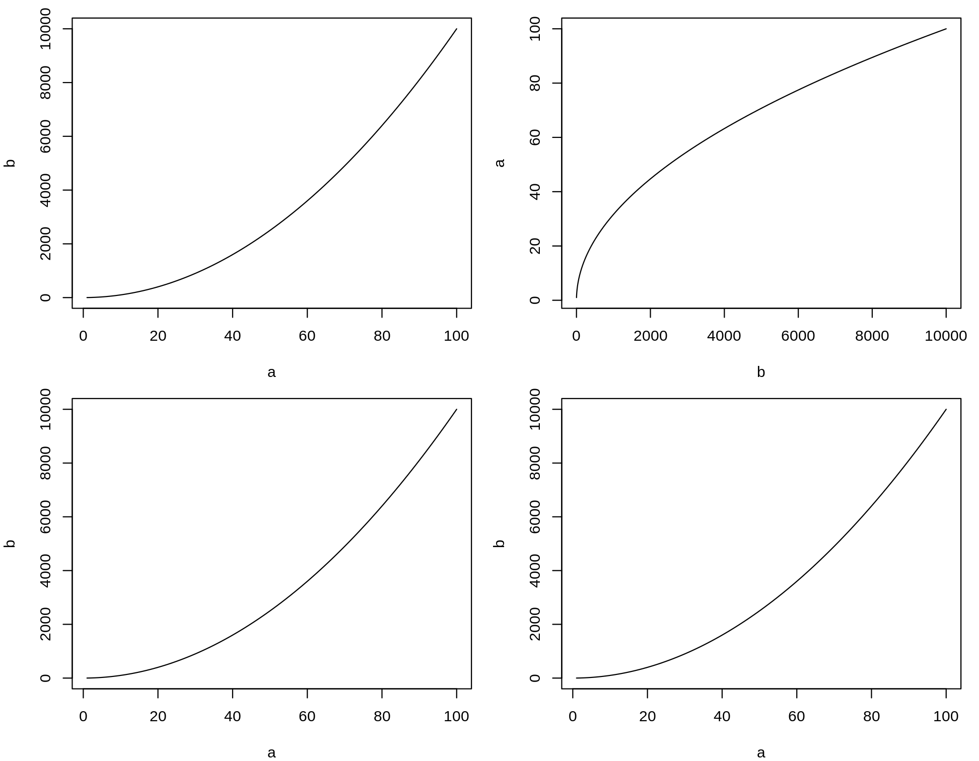
Challenge
plot is a function that draws a graph of y as a function of x. It requires two arguments names x and y. What are the differences between the following lines?
a <- 1:100b <- a^2plot(a, b, type = "l")plot(b, a, type = "l")plot(x = a, y = b, type = "l")plot(y = b, x = a, type = "l")The argument type of the function plot let you choose the type of graph you want. Try it without this argument.
Challenge: Solution
plot is a function that draws a graph of y as a function of x. It requires two arguments names x and y. What are the differences between the following lines?
Challenge: Solution
plot(a, b, type = "l")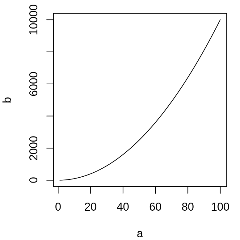
plot(b, a, type = "l")
The shape of the plot changes, as we did not provide the argument's names, the order is important.
Challenge: Solution
plot(x = a, y = b, type = "l")
plot(y = b, x = a, type = "l")
Same as plot(a, b, type = "l"). The argument names are provided, the order is not important.
Loading your first R package: ggplot2
We need to gain access the functions that are available within the installed package. To do this, load ggplot2 using the library() function.
library(ggplot2)Now we can draw the graph
qplot(1:10, 1:10)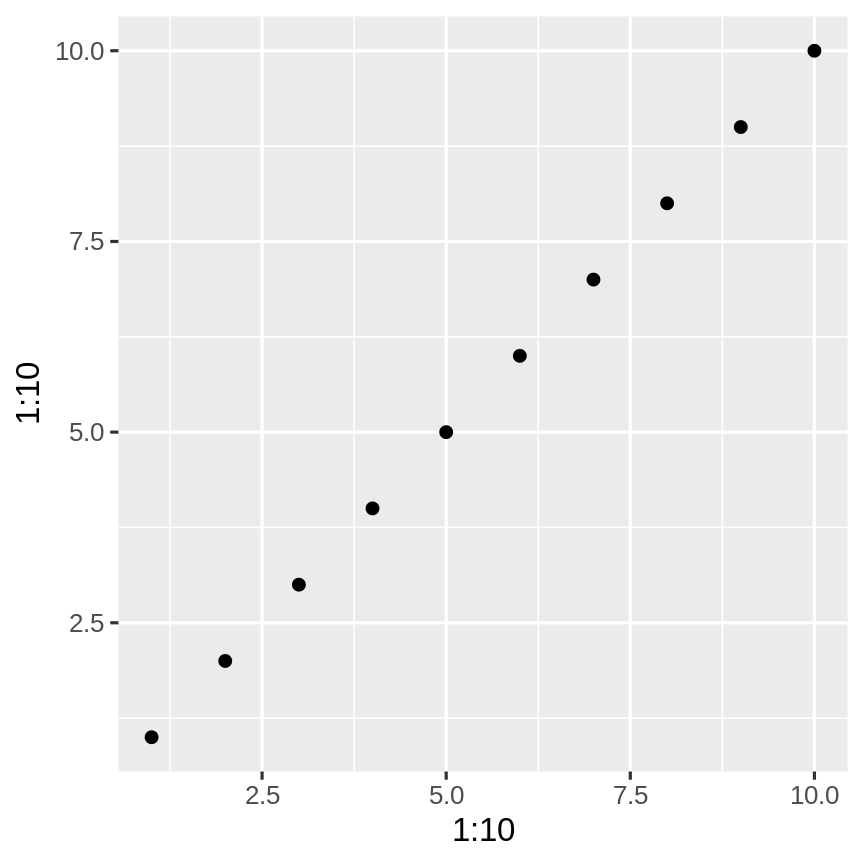
The ggplot2 package will be covered in Workshop #3: Introduction to ggplot2.
Search results

Search results

Search results

Help pages
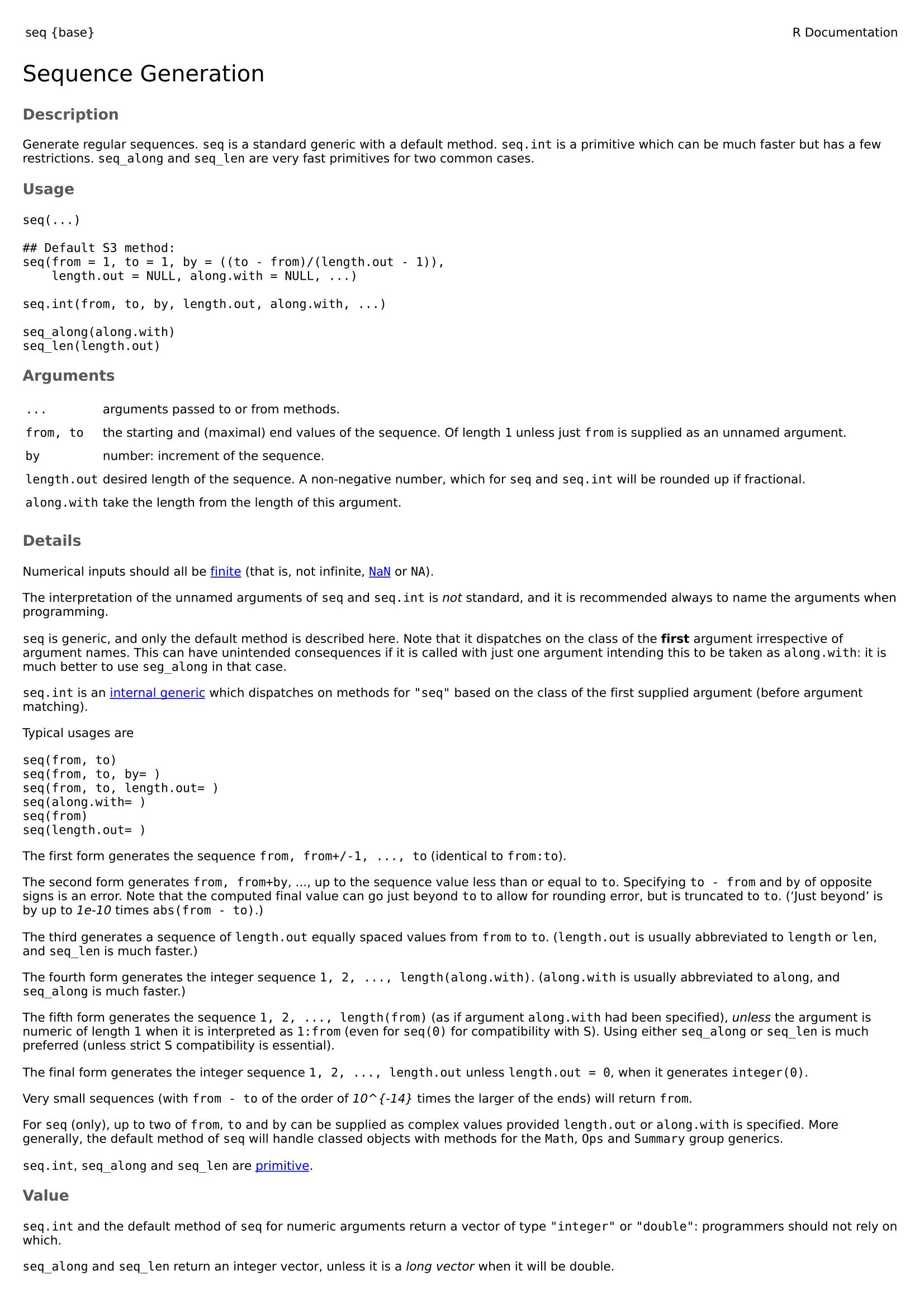
Description
function_name {package_name}Description: a short description of what the function does.
Usage
- How to call the function
- If
name = valueis present, a default value is provided if the argument is missing. The argument becomes optional. - Other related functions described in this help page
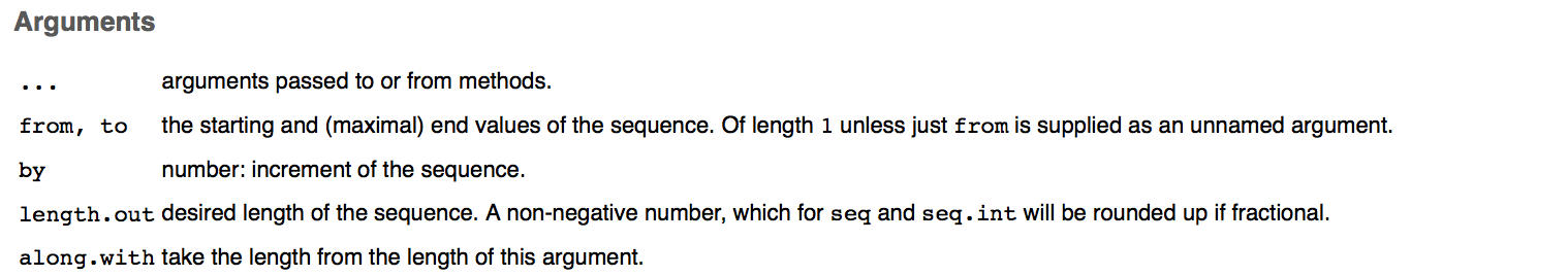
Arguments
- Description of all the arguments and what they are used for
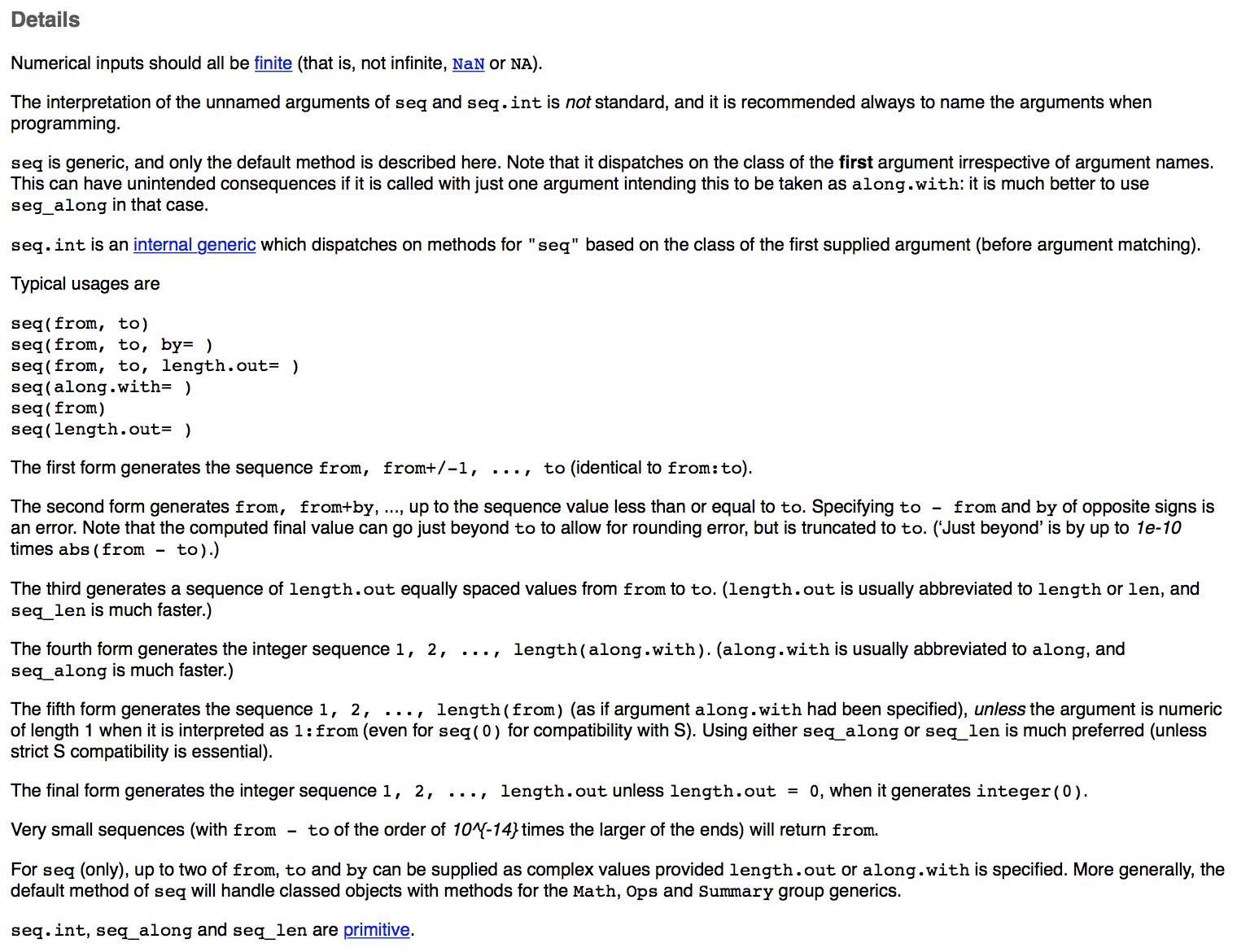
Details
- A detailed description of how the functions work and their characteristics
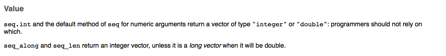
Value, See Also, and Examples
- A description of the return value
Value, See Also, and Examples
- A description of the return value
- Other related functions that can be useful
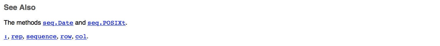
Value, See Also, and Examples
- A description of the return value
- Other related functions that can be useful
- Reproducible examples
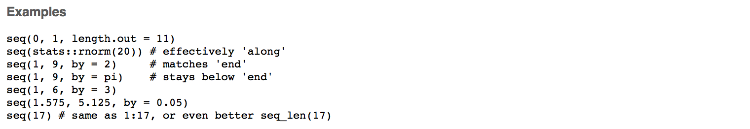
Challenge
Create a sequence of even numbers from 0 to 10 using the
seqfunction.Create an unsorted vector of your favourite numbers, then sort your vector in reverse order.
Challenge: Solutions
- Create a sequence of even numbers from 0 to 10 using the
seqfunction.
seq(from = 0, to = 10, by = 2)# [1] 0 2 4 6 8 10seq(0, 10, 2)# [1] 0 2 4 6 8 10- Create an unsorted vector of your favorite numbers, then sort your vector in reverse order.
numbers <- c(2, 4, 22, 6, 26)sort(numbers, decreasing = TRUE)# [1] 26 22 6 4 2Challenge
Find the appropriate functions to perform the following operations:
- Square root
- Calculate the mean of numbers
- Combine two data frames by columns
- List available objects in your workspace
Challenge: Solutions
Find the appropriate functions to perform the following operations:
- Square root
sqrt()
- Calculate the mean of numbers
mean()
- Combine two data frames by columns
cbind()
- List available objects in your workspace
ls()
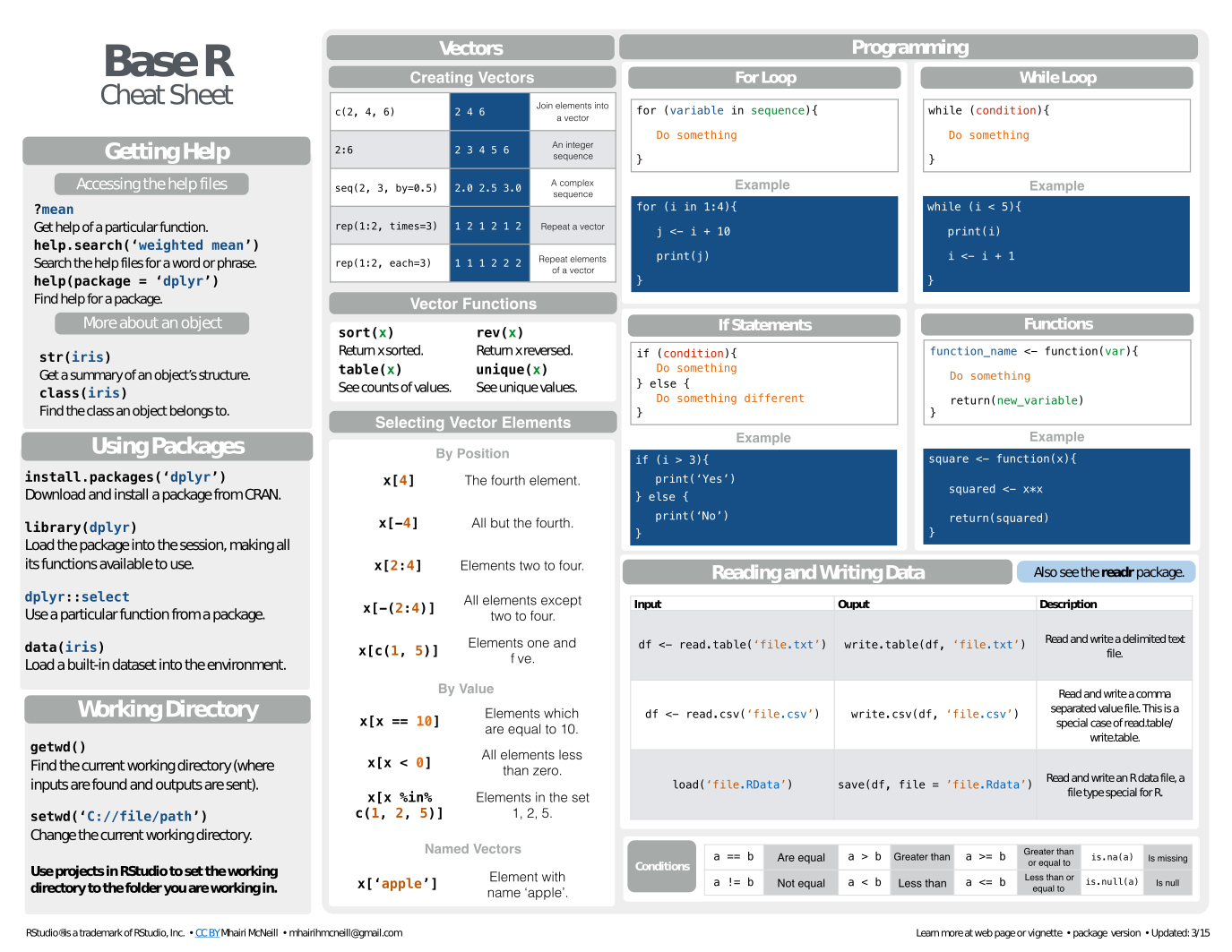
Cheat 4ever

Lots of cheat sheets are available online.
Open it directly from RStudio: Help → Cheatsheets
Cheatsheet 4ever
Some useful R books

Thank you for attending!
![]()