class: center, middle, inverse, title-slide # Workshop 5: Programming in R ## QCBS R Workshop Series ### Québec Centre for Biodiversity Science --- ## Outline 1. Learning what is **control flow** 2. Writing your first functions in R 3. Speeding up your code 4. Useful R packages for biologists --- class: inverse, center, middle # Review --- ## Objects 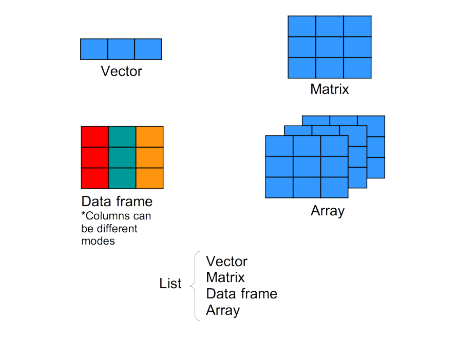 --- ## Vectors Numeric vectors ```r num.vector <- c(1, 4, 3, 98, 32, -76, -4) ``` ```r num.vector # [1] 1 4 3 98 32 -76 -4 ``` --- ## Data frames vectors ```r siteID <- c("A1.01", "A1.02", "B1.01", "B1.02") soil_pH <- c(5.6, 7.3, 4.1, 6.0) num.sp <- c(17, 23, 15, 7) treatment <- c("Fert", "Fert", "No_fert", "No_fert") ``` We then combine them using the function `data.frame` ```r my.first.df <- data.frame(siteID, soil_pH, num.sp, treatment) ``` ```r my.first.df # siteID soil_pH num.sp treatment # 1 A1.01 5.6 17 Fert # 2 A1.02 7.3 23 Fert # 3 B1.01 4.1 15 No_fert # 4 B1.02 6.0 7 No_fert ``` --- ## Lists ```r my.first.list <- list(siteID, soil_pH, num.sp, treatment) ``` ```r my.first.list # [[1]] # [1] "A1.01" "A1.02" "B1.01" "B1.02" # # [[2]] # [1] 5.6 7.3 4.1 6.0 # # [[3]] # [1] 17 23 15 7 # # [[4]] # [1] "Fert" "Fert" "No_fert" "No_fert" ``` --- class: inverse, center, middle # Control flow --- ## Control flow Program flow control can be simply defined as the order in which a program is executed. #### Why is it advantageous to have structured programs? - It **decreases the complexity** and time of the task at hand; - This logical structure also means that the code has **increased clarity**; - It also means that **many programmers can work on one program**. .large[.center[**This means increased productivity**]] --- ## Control flow Flowcharts can be used to plan programs and represent their structure <br> 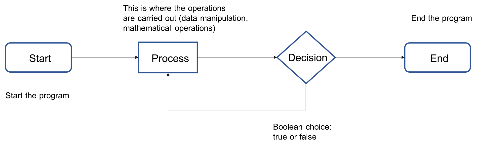 --- ## Representing structure The two basic building blocks of codes are the following: .pull-left[ #### Selection Program's execution determined by statements ```r if if else ``` ] .pull-right[ #### Iteration Repetition, where the statement will **loop** until a criteria is met ```r for while repeat ``` ] --- ## Decision making .pull-left[ **`if` statement** ```R if(condition) { expression } ``` .center[ 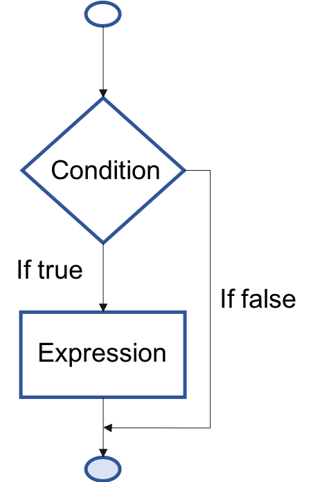 ] ] .pull-right[ **`if` `else` statement** ```r if(condition) { expression 1 } else { expression 2 } ``` .center[ 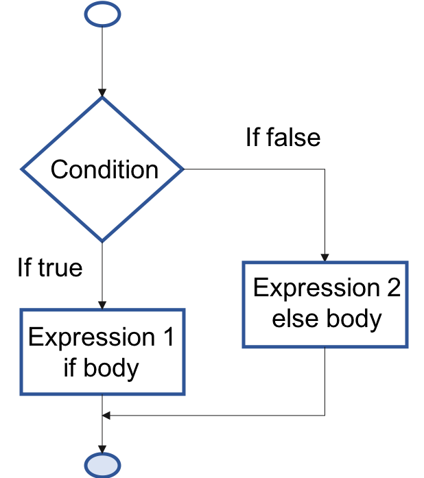 ] ] --- #### What if you want to test more than one condition? - `if` and `if` `else` test a single condition - You can also use `ifelse` function to: - test a vector of conditions; - apply a function only under certain conditions. ```r a <- 1:10 ifelse(a > 5, "yes", "no") a <- (-4):5 sqrt(ifelse(a >= 0, a, NA)) ``` --- ## Nested `if` `else` statement .small[ ```r if (test_expression1) { statement1 } else if (test_expression2) { statement2 } else if (test_expression3) { statement3 } else { statement4 } ``` ] .center[ ] --- ## Challenge 1 ![:cube]() ```r Paws <- "cat" Scruffy <- "dog" Sassy <- "cat" animals <- c(Paws, Scruffy, Sassy) ``` 1. Use an `if` statement to print “meow” if `Paws` is a “cat”. 2. Use an `if` `else` statement to print `“woof”` if you supply an object that is a `“dog”` and `“meow”` if it is not. Try it out with `Paws` and `Scruffy`. 3. Use the `ifelse` function to display `“woof”` for `animals` that are dogs and `“meow”` for `animals` that are cats. --- ## Challenge 1 - Solution ![:cube]() 1- Use an `if` statement to print “meow” if `Paws` is a “cat”. ```r if(Paws == 'cat') { print("meow") } # [1] "meow" ``` 2- Use an `if` `else` statement to print `“woof”` if you supply an object that is a `“dog”` and `“meow”` if it is not. Try it out with `Paws` and `Scruffy`. ```r x = Paws # x = Scruffy if(x == 'cat') { print("meow") } else { print("woof") } # [1] "meow" ``` --- ## Challenge 1 - Solution ![:cube]() 3- Use the `ifelse` function to display `“woof”` for `animals` that are dogs and `“meow”` for `animals` that are cats. ```r animals <- c(Paws, Scruffy, Sassy) ifelse(animals == 'dog', "woof", "meow") # [1] "meow" "woof" "meow" ``` Or ```r for(val in 1:3) { if(animals[val] == 'cat') { print("meow") }else if(animals[val] == 'dog') { print("woof") }else print("what?") } # [1] "meow" # [1] "woof" # [1] "meow" ``` --- ## Beware of R’s expression parsing! Use curly brackets `{}` so that R knows to expect more input. Try: ```r if (2+2) == 4 print("Arithmetic works.") else print("Houston, we have a problem.") ``` .center[.alert[This doesn't work because R evaluates the first line and doesn't know that you are going to use an `else` statement]] Instead use: ```r *if (2+2 == 4) { print("Arithmetic works.") *} else { print("Houston, we have a problem.") *} # [1] "Arithmetic works." ``` --- ## Remember the logical operators | Command | Meaning | | :-------------: | :-------------: | | `==` | equal to | | `!=` | not x | | `<` | less than | | `<=` | less than or equal to | | `>` | greater than | | `>=` | greater than or equal to | | `x&y` | x AND y | | `x`&#124;`y` | x OR y | | `isTRUE(x)` | test if X is true | --- ## Iteration Every time some operations have to be repeated, a loop may come in handy Loops are good for: - doing something for every element of an object - doing something until the processed data runs out - doing something for every file in a folder - doing something that can fail, until it succeeds - iterating a calculation until it converges --- ## `for` loop A `for` loop works in the following way: ```R for(val in sequence) { statement } ``` .center[  ] --- ## `for` loop The letter `i` can be replaced with any variable name and the sequence can be almost anything, even a list of vectors. ```r # Try the commands below and see what happens: for (a in c("Hello", "R", "Programmers")) { print(a) } for (z in 1:30) { a <- rnorm(n = 1, mean = 5, sd = 2) print(a) } elements <- list(1:3, 4:10) for (element in elements) { print(element) } ``` --- ## `for` loop In the example below, R would evaluate the expression 5 times: ```r for(i in 1:5) { expression } ``` In the example, every instance of `m` is being replaced by each number between `1:10`, until it reaches the last element of the sequence. .pull-left[ ```r for(m in 1:10) { print(m*2) } ``` ] .small[ .pull-right[.pull-left[ ``` # [1] 2 # [1] 4 # [1] 6 # [1] 8 # [1] 10 ``` ] .pull-right[ ``` # [1] 12 # [1] 14 # [1] 16 # [1] 18 # [1] 20 ``` ] ] ] --- ## `for` loop .small[ ```r x <- c(2,5,3,9,6) count <- 0 for (val in x) { if(val %% 2 == 0) { count = count+1 } } print(count) ``` ] .center[  ] --- ## `for` loop For loops are often used to loop over a dataset. We will use loops to perform functions on the `CO2` dataset which is built in R. ```R data(CO2) # This loads the built in dataset for (i in 1:length(CO2[,1])) { # for each row in the CO2 dataset print(CO2$conc[i]) # print the CO2 concentration } for (i in 1:length(CO2[,1])) { # for each row in the CO2 dataset if(CO2$Type[i] == "Quebec") { # if the type is "Quebec" print(CO2$conc[i]) # print the CO2 concentration } } ``` --- ## `for` loop .alert[Tip 1]. To loop over the number of rows of a data frame, we can use the function `nrow()` ```r for (i in 1:nrow(CO2)) { # for each row in the CO2 dataset print(CO2$conc[i]) # print the CO2 concentration } ``` .alert[Tip 2]. If we want to perform operations on the elements of one column, we can directly iterate over it ```r for (p in 1:CO2$conc) { # for each row of the column "conc"of the CO2 df print(p) # print the p-th element } ``` --- ## `for` loop The expression within the loop can be almost anything and is usually a compound statement containing many commands. ```r for (i in 4:5) { # for i in 4 to 5 print(colnames(CO2)[i]) print(mean(CO2[,i])) # print the mean of that column from the CO2 dataset } ``` Output: ``` # [1] "conc" # [1] 435 # [1] "uptake" # [1] 27.2131 ``` --- ## `for` loops within `for` loops In some cases, you may want to use nested loops to accomplish a task. When using nested loops, it is important to use different variables as counters for each of your loops. Here we used `i` and `n`: .pull-left[ ```r for (i in 1:3) { for (n in 1:3) { print (i*n) } } ``` ] .pull-right[ ```r # Output # [1] 1 # [1] 2 # [1] 3 # [1] 2 # [1] 4 # [1] 6 # [1] 3 # [1] 6 # [1] 9 ``` ] --- ## Getting good: using the `apply()` family R disposes of the `apply()` function family, which consists of vectorized functions that aim at **minimizing your need to explicitly create loops**. `apply()` can be used to apply functions to a matrix. .pull-left[ ```r (height <- matrix(c(1:10, 21:30), nrow = 5, ncol = 4)) # [,1] [,2] [,3] [,4] # [1,] 1 6 21 26 # [2,] 2 7 22 27 # [3,] 3 8 23 28 # [4,] 4 9 24 29 # [5,] 5 10 25 30 ``` ] .pull-right[ ```r apply(X = height, MARGIN = 1, FUN = mean) # [1] 13.5 14.5 15.5 16.5 17.5 ``` ```r ?apply ``` ] --- ## `lapply()` `lapply()` applies a function to every element of a `list`. It may be used for other objects like **dataframes**, **lists** or **vectors**. The output returned is a `list` (explaining the “`l`” in `lapply`) and has the same number of elements as the object passed to it. .pull-left[ ```r SimulatedData <- list( SimpleSequence = 1:4, Norm10 = rnorm(10), Norm20 = rnorm(20, 1), Norm100 = rnorm(100, 5)) # Apply mean to each element ## of the list lapply(SimulatedData, mean) ``` ] .small[ .pull-right[ ``` # $SimpleSequence # [1] 2.5 # # $Norm10 # [1] 0.1189506 # # $Norm20 # [1] 1.284905 # # $Norm100 # [1] 5.092327 ``` ] ] --- ## `sapply()` `sapply()` sapply() is a ‘wrapper’ function for `lapply()`, but returns a simplified output as a `vector`, instead of a `list`. The output returned is a `list` (explaining the “`l`” in `lapply`) and has the same number of elements as the object passed to it. .small[ ```r SimulatedData <- list(SimpleSequence = 1:4, Norm10 = rnorm(10), Norm20 = rnorm(20, 1), Norm100 = rnorm(100, 5)) ``` ```r # Apply mean to each element of the list sapply(SimulatedData, mean) # SimpleSequence Norm10 Norm20 Norm100 # 2.5000000 -0.5253051 1.4559801 5.2008865 ``` ] --- ## `mapply()` `mapply()` works as a multivariate version of `sapply()`. It will apply a given function to the first element of each argument first, followed by the second element, and so on. For example: ```r lilySeeds <- c(80, 65, 89, 23, 21) poppySeeds <- c(20, 35, 11, 77, 79) ``` ```r # Output mapply(sum, lilySeeds, poppySeeds) # [1] 100 100 100 100 100 ``` --- ## `tapply()` `tapply()` is used to apply a function over subsets of a vector. It is primarily used when the dataset contains dataset contains different groups (*i*.*e*. levels/factors) and we want to apply a function to each of these groups. ```r head(mtcars) # mpg cyl disp hp drat wt qsec vs am gear carb # Mazda RX4 21.0 6 160 110 3.90 2.620 16.46 0 1 4 4 # Mazda RX4 Wag 21.0 6 160 110 3.90 2.875 17.02 0 1 4 4 # Datsun 710 22.8 4 108 93 3.85 2.320 18.61 1 1 4 1 # Hornet 4 Drive 21.4 6 258 110 3.08 3.215 19.44 1 0 3 1 # Hornet Sportabout 18.7 8 360 175 3.15 3.440 17.02 0 0 3 2 # Valiant 18.1 6 225 105 2.76 3.460 20.22 1 0 3 1 ``` ```r # get the mean hp by cylinder groups tapply(mtcars$hp, mtcars$cyl, FUN = mean) # 4 6 8 # 82.63636 122.28571 209.21429 ``` --- ## Challenge 2 ![:cube]() You have realized that your tool for measuring uptake was not calibrated properly at Quebec sites and all measurements are 2 units higher than they should be. 1. Use a loop to correct these measurements for all Quebec sites. 2. Use a vectorisation-based method to calculate the mean CO2-uptake in both areas. For this, you will have to load the CO2 dataset using `data(CO2)`, and then use the object `CO2`. --- ## Challenge 2: Solution ![:cube]() 1. Using `for` and `if` to correct the measurements: ```r for (i in 1:dim(CO2)[1]) { if(CO2$Type[i] == "Quebec") { CO2$uptake[i] <- CO2$uptake[i] - 2 } } ``` 2. Using `tapply()` to calculate the mean for each group: ```r tapply(CO2$uptake, CO2$Type, mean) # Quebec Mississippi # 31.54286 20.88333 ``` --- ## Modifying iterations Normally, loops iterate over and over until they finish. Sometimes you may be interested in breaking this behaviour. For example, you may want to tell R to stop executing the iteration when it reaches a given element or condition. You may also want R to jump certain elements when certain conditions are met. For this, we will introduce `break`, `next` and `while`. --- ## Modifying iterations: `break` ```r for(val in x) { if(condition) { break } statement } ```  --- ## Modifying iterations: `next` ```r for(val in x) { if(condition) { next } statement } ```  --- ## Modifying iterations: `next` Print the `\(CO_{2}\)` concentrations for "chilled" treatments and keep count of how many replications were done. ```r count <- 0 for (i in 1:nrow(CO2)) { if (CO2$Treatment[i] == "nonchilled") next # Skip to next iteration if treatment is nonchilled count <- count + 1 # print(CO2$conc[i]) } print(count) # The count and print command were performed 42 times. ``` ``` # [1] 42 ``` ```r sum(CO2$Treatment == "nonchilled") # [1] 42 ``` --- ## Modifying iterations: `break` This could be equivalently written using a `repeat` loop and `break`: ```r count <- 0 i <- 0 repeat { i <- i + 1 if (CO2$Treatment[i] == "nonchilled") next # skip this loop count <- count + 1 print(CO2$conc[i]) if (i == nrow(CO2)) break # stop looping } print(count) ``` --- ## Modifying iterations: `while` This could also be written using a `while` loop: ```r i <- 0 count <- 0 while (i < nrow(CO2)) { i <- i + 1 if (CO2$Treatment[i] == "nonchilled") next # skip this loop count <- count + 1 print(CO2$conc[i]) } print(count) ``` --- ## Challenge 3 ![:cube]() You have realized that your tool for measuring concentration did not work properly. At Mississippi sites, concentrations less than 300 were measured correctly, but concentrations equal or higher than 300 were overestimated by 20 units! Your *mission* is to use a loop to correct these measurements for all Mississippi sites. .alert[Tip]. Make sure you reload the data so that we are working with the raw data for the rest of the exercise: ```r data(CO2) ``` --- ## Challenge 3: Solution ![:cube]() ```r for (i in 1:nrow(CO2)) { if(CO2$Type[i] == "Mississippi") { if(CO2$conc[i] < 300) next CO2$conc[i] <- CO2$conc[i] - 20 } } ``` .comment[Note: We could also have written it in this way, which is more concise and clear:] ```r for (i in 1:nrow(CO2)) { if(CO2$Type[i] == "Mississippi" && CO2$conc[i] >= 300) { CO2$conc[i] <- CO2$conc[i] - 20 } } ``` --- ## Edit a plot using `for` and `if` Let's plot **uptake** vs **concentration** with points of different colors according to their type (*Quebec* or *Mississippi*) and **treatment** (*chilled* or *nonchilled*). .small[ ```r plot(x = CO2$conc, y = CO2$uptake, type = "n", cex.lab=1.4, xlab = "CO2 concentration", ylab = "CO2 uptake") # Type "n" tells R to not actually plot the points. for (i in 1:length(CO2[,1])) { if (CO2$Type[i] == "Quebec" & CO2$Treatment[i] == "nonchilled") { points(CO2$conc[i], CO2$uptake[i], col = "red") } if (CO2$Type[i] == "Quebec" & CO2$Treatment[i] == "chilled") { points(CO2$conc[i], CO2$uptake[i], col = "blue") } if (CO2$Type[i] == "Mississippi" & CO2$Treatment[i] == "nonchilled") { points(CO2$conc[i], CO2$uptake[i], col = "orange") } if (CO2$Type[i] == "Mississippi" & CO2$Treatment[i] == "chilled") { points(CO2$conc[i], CO2$uptake[i], col = "green") } } ``` ] --- ## Challenge 4 ![:cube]() <br> Create a plot using `for` loop and `if` <img src="workshop05-en_files/figure-html/unnamed-chunk-39-1.png" width="504" style="display: block; margin: auto;" /> --- ## Challenge 4![:cube]() <br> <br> Generate a plot showing **concentration versus uptake** where each plant is shown using a different .alert[colour] point. .alert[Bonus points] for doing it with nested loops! .comment[Steps: <br> 1. Create an empty plot <br> 2. Create a list of plants (hint: `?unique`) <br> 3. Fill the plot using `for` and `if` statements] --- ## Challenge 4: Solution ![:cube]() .small[ ```r plot(x = CO2$conc, y = CO2$uptake, type = "n", cex.lab=1.4, xlab = "CO2 concentration", ylab = "CO2 uptake") plants <- unique(CO2$Plant) for (i in 1:nrow(CO2)){ for (p in 1:length(plants)) { if (CO2$Plant[i] == plants[p]) { points(CO2$conc[i], CO2$uptake[i], col = p) }}} ``` <img src="workshop05-en_files/figure-html/unnamed-chunk-40-1.png" width="432" style="display: block; margin: auto;" /> ] --- class: inverse, center, middle # Writing functions --- ## Why write functions? Much of the heavy lifting in R is done by functions. They are useful for: 1. Performing a task repeatedly, but configurably; 2. Making your code more readable; 3. Make your code easier to modify and maintain; 4. Sharing code between different analyses; 5. Sharing code with other people; 6. Modifying R’s built-in functionality. --- ## What is a function? <br> <br> .center[  ] --- ## Syntax of a function ```r function_name <- function(argument1, argument2, ...) { expression... # What we want the function to do return(value) # Optional } ``` --- ## Arguments of a function ```r function_name <- function(argument1, argument2, ...) { expression... return(value) } ``` Arguments are the entry values of your function and will have the information your function needs to be able to perform correctly. A function can have between 0 and an infinity of arguments. See the following example: .small[ ```r operations <- function(number1, number2, number3) { result <- (number1 + number2) * number3 print(result) } ``` ```r operations(1, 2, 3) # [1] 9 ``` ] --- ## Challenge 5 ![:cube]() Using what you learned previously on flow control, create a function `print_animal` that takes an `animal` as argument and gives the following results: ```r Scruffy <- "dog" Paws <- "cat" print_animal(Scruffy) # [1] "woof" print_animal(Paws) # [1] "meow" ``` --- ## Challenge 5: Solution ![:cube]() <br> <br> ```r print_animal <- function(animal) { if (animal == "dog") { print("woof") } else if (animal == "cat") { print("meow") } } ``` --- ## Default values in a function Arguments can also be optional and be provided with a default value. This is useful when using a function with the same settings, but still provides the flexibility to change its values, if needed. ```r operations <- function(number1, number2, number3 = 3) { result <- (number1 + number2) * number3 print(result) } operations(1, 2, 3) # is equivalent to # [1] 9 operations(1, 2) # [1] 9 operations(1, 2, 2) # we can still change the value of number3 if needed # [1] 6 ``` --- ## Argument `...` The special argument `...` allows you to pass on arguments to another function used inside your function. Here we use `...` to pass on arguments to `plot()` and `points()`. ```r plot.CO2 <- function(CO2, ...) { * plot(x=CO2$conc, y=CO2$uptake, type="n", ...) for (i in 1:length(CO2[,1])){ if (CO2$Type[i] == "Quebec") { * points(CO2$conc[i], CO2$uptake[i], col = "red", type = "p", ...) } else if (CO2$Type[i] == "Mississippi") { * points(CO2$conc[i], CO2$uptake[i], col = "blue", type = "p", ...) } } } plot.CO2(CO2, cex.lab=1.2, xlab="CO2 concentration", ylab="CO2 uptake") plot.CO2(CO2, cex.lab=1.2, xlab="CO2 concentration", ylab="CO2 uptake", pch=20) ``` --- ## Argument `...` The special argument `...` allows you to pass on arguments to another function used inside your function. Here we use `...` to pass on arguments to `plot()` and `points()`. <img src="workshop05-en_files/figure-html/unnamed-chunk-47-1.png" width="720" style="display: block; margin: auto;" /> --- ## Argument `...` The special argument `...` allows you to input an indefinite number of arguments. ```r sum2 <- function(...){ * args <- list(...) result <- 0 for (i in args) { result <- result + i } return (result) } sum2(2, 3) # [1] 5 sum2(2, 4, 5, 7688, 1) # [1] 7700 ``` --- ## Return values The last expression evaluated in a `function` becomes the return value. ```r myfun <- function(x) { if (x < 10) { 0 } else { 10 } } myfun(5) # [1] 0 myfun(15) # [1] 10 ``` .comment[`function()` itself returns the last evaluated value even without including `return()` function.] --- ## Return values .small[ It can be useful to explicitly `return()` if the routine should end early, jump out of the function and return a value. ```r simplefun1 <- function(x) { if (x<0) return(x) } ``` Functions can return only a single object (and text). But this is not a limitation because you can return a `list` containing any number of objects. .pull-left[ ```r simplefun2 <- function(x, y) { z <- x + y return(list("result" = z, "x" = x, "y" = y)) } ``` ] .pull-right[ .pull-left[ <br> ```r simplefun2(1, 2) ``` ] .pull-right[ ``` # $result # [1] 3 # # $x # [1] 1 # # $y # [1] 2 ``` ] ] ] --- ## Challenge 6 ![:cube]() <br> Using what you have just learned on functions and control flow, create a function named `bigsum` that takes two arguments `a` and `b` and: 1. Returns 0 if the sum of `a` and `b` is strictly less than 50; 2. Else, returns the sum of `a` and `b`. --- ## Challenge 6: Solution ![:cube]() <br><br> .pull-left[ **Answer 1** ```r bigsum <- function(a, b) { result <- a + b if (result < 50) { return(0) } else { return (result) } } ``` ] .pull-right[ **Answer 2** ```r bigsum <- function(a, b) { result <- a + b if (result < 50) { 0 } else { result } } ``` ] --- ## Accessibility of variables It is essential to always keep in mind where your variables are, and whether they are defined and accessible:  Variables defined .alert[inside] a function are not accessible outside of it!  Variables defined .alert[outside] a function are accessible inside. But it is NEVER a good idea, as your function will not function if the outside variable is erased. --- ## Accessibility of variables ```r var1 <- 3 # var1 is defined outside our function vartest <- function() { a <- 4 # 'a' is defined inside print(a) # print 'a' print(var1) # print var1 } a # we cannot print 'a' as it exists only inside the function # Error in eval(expr, envir, enclos): object 'a' not found vartest() # calling vartest() will print a and var1 # [1] 4 # [1] 3 rm(var1) # remove var1 vartest() # calling the function again doesn't work anymore # [1] 4 # Error in print(var1): object 'var1' not found ``` --- ## Accessibility of variables .alert[Mandatory tip.] Use arguments then! Also, inside a function, arguments names will take over other variable names. ```r var1 <- 3 # var1 is defined outside our function vartest <- function(var1) { print(var1) # print var1 } vartest(8) # Inside our function var1 is now our argument and takes its value # [1] 8 var1 # var1 still has the same value # [1] 3 ``` --- ## Accessibility of variables .pull-left[ .alert[Tip.] Be very careful when creating variables inside a conditional statement as the variable may never have been created and cause (sometimes imperceptible) errors. <br> <br> <br> .alert[Tip.] It is good practice to define variables outside the conditions and then modify their values to avoid any problem ] .small[ .pull-right[ ```r a <- 3 if (a > 5) { b <- 2 } a + b ``` ```r # Error: object 'b' not found ``` .small[If you had `b` already assigned in your environment, with a different value, you could have had a .alert[bigger] problem! No error would have been shown and `a + b` would have meant another thing!] ] ] --- class: inverse, center, middle # Good programming practices --- ## Why should I care about programming practices? - To make your life easier; - To achieve greater readability and makes sharing and reusing your code a lot less painful; - To reduce the time you will spend to understand your code. .center[.large[Pay attention to the next tips!]] --- ## Keep a clean and nice code Proper indentation and spacing is the first step to get an easy to read code: - Use **spaces** between and after you operators; - Use consistentely the same assignation operator. `<-` is often preferred. `=` is OK, but do not switch all the time between the two; - Use brackets when using flow control statements: <br> - Inside brackets, indent by *at least* two spaces; - Put closing brackets on a separate line, except when preceding an `else` statement. <br> - Define each variable on its own line. --- ## Keep a clean and nice code On the left, code is not spaced. All brackets are in the same line, and it looks "messy". .small[ .pull-left[ ```r a<-4;b=3 if(a<b){ if(a==0)print("a zero")}else{ if(b==0){print("b zero")}else print(b)} ``` ] ] --- ## Keep a clean and nice code On the left, code is not spaced. All brackets are in the same line, and it looks "messy". On the right, it looks more organized, no? .small[ .pull-left[ ```r a<-4;b=3 if(a<b){ if(a==0)print("a zero")}else{ if(b==0){print("b zero")}else print(b)} ``` ] .pull-right[ ```r a <- 4 b <- 3 if(a < b){ if(a == 0) { print("a zero") } } else { if(b == 0){ print("b zero") } else { print(b) } } ``` ] ] --- ## Use functions to simplify your code Write your own function: 1. When portion of the code is repeated more than twice in your script; 2. If only a part of the code changes and includes options for different arguments. This would also reduce the number of potential errors done by copy-pasting, and the time needed to correct them. --- ## Use functions to simplify your code Let's modify the example from **Challenge #3** and suppose that all `\(CO_2\)` uptake from Mississipi plants was overestimated by 20 and Quebec underestimated by 50. .small[ .pull-left[ We could write this: <br> ```r for (i in 1:length(CO2[,1])) { if(CO2$Type[i] == "Mississippi") { CO2$conc[i] <- CO2$conc[i] - 20 } } for (i in 1:length(CO2[,1])) { if(CO2$Type[i] == "Quebec") { CO2$conc[i] <- CO2$conc[i] + 50 } } ``` ] .pull-right[ Or this: ```r recalibrate <- function(CO2, type, bias){ for (i in 1:nrow(CO2)) { if(CO2$Type[i] == type) { CO2$conc[i] <- CO2$conc[i] + bias } } return(CO2) } ``` .small[ ```r newCO2 <- recalibrate(CO2, "Mississipi", -20) newCO2 <- recalibrate(newCO2, "Quebec", +50) ``` ] ] ] --- ## Use meaningful names for functions Same function as before, but with vague names. .pull-left[ ```r rc <- function(c, t, b) { for (i in 1:nrow(c)) { if(c$Type[i] == t) { c$uptake[i] <- c$uptake[i] + b } } return (c) } ``` ] .pull-right[ <br> <br> .center[.alert[What is `c` and `rc`?]]] .comment[Whenever possible, avoid using names of existing `R` functions and variables to avoid confusion and conflits.] --- ## Use comments .alert[Final tip]. Add comment to describe what your code does, how to use its arguments or a detailed step-by-step description of the function. .small[ ```r # Recalibrates the CO2 dataset by modifying the CO2 uptake concentration # by a fixed amount depending on the region of sampling # Arguments # CO2: the CO2 dataset # type: the type ("Mississippi" or "Quebec") that need to be recalibrated. # bias: the amount to add or remove to the concentration uptake recalibrate <- function(CO2, type, bias) { for (i in 1:nrow(CO2)) { if(CO2$Type[i] == type) { CO2$uptake[i] <- CO2$uptake[i] + bias } } return(CO2) } ``` ] --- class: inverse, center, bottom # Thank you for attending this workshop!